1. Quick Start
1.1. Installation from Github
To install the py-lmd library you can use pip.
pip install py-lmd
Once installed the modules can be loaded as following:
from lmd.lib import Collection, Shape
1.2. Generating Shapes
As first example we will create a cutting data for a rectangle and visualize it. First we need to think of a calibration points for our coordinate system. The calibration points are specified as Numpy array and should have the shape (3, 2). When calibrating the file on the Leica LMD after loading the file, the order of selecting the calibration points is the same as the order of points set here. If no other orientation transform has been specified, the calibration points are defined in the (x, y) coordinate system. More on the usage of different coordinate systems can be found under XXX.
import numpy as np
from lmd.lib import Collection, Shape

calibration = np.array([[0, 0],
                        [0, 100],
                        [50, 50]])
With these calibration coordinates we can create our Collection object. The Collection is the base object for creating cutting data and holds a list of Shape objects. Furthermore, it allows to read and write the Leica LMD XML format and handles the coordinate system.
my_first_collection = Collection(calibration_points = calibration)
We can then create our first rectangle by using the Shape object and passing it to our collection by using the add_shape method. For creating the Shape object we need to pass the vertices as Numpy array. List of vertices should always be closed with the last vertex equaling the first one.
rectangle_coordinates = np.array([[10,10],
                                  [40,10],
                                  [40,40],
                                  [10,40],
                                  [10,10]])
rectangle = Shape(rectangle_coordinates)
my_first_collection.add_shape(rectangle)
We can visualize our collection with the plot method. Using the calibration = True parameter will include the calibration coordinates in the plot.
my_first_collection.plot(calibration = True)
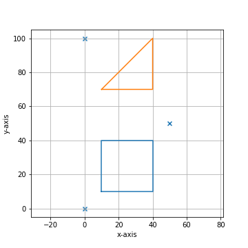
We can generate a second shape in form of a triangle. This time we will be using the new_shape method of the collection object.
triangle_coordinates = np.array([[10,70], [40,70], [40,100], [10,70]])
my_first_collection.new_shape(triangle_coordinates)

my_first_collection.plot(calibration = True)
We can then export and save our collection of shapes into xml cutting data.
my_first_collection.save("first_collection.xml")
<?xml version='1.0' encoding='UTF-8'?>
<ImageData>
  <GlobalCoordinates>1</GlobalCoordinates>
  <X_CalibrationPoint_1>0</X_CalibrationPoint_1>
  <Y_CalibrationPoint_1>0</Y_CalibrationPoint_1>
  <X_CalibrationPoint_2>0</X_CalibrationPoint_2>
  <Y_CalibrationPoint_2>10000</Y_CalibrationPoint_2>
  <X_CalibrationPoint_3>5000</X_CalibrationPoint_3>
  <Y_CalibrationPoint_3>5000</Y_CalibrationPoint_3>
  <ShapeCount>2</ShapeCount>
  <Shape_1>
    <PointCount>5</PointCount>
    <X_1>1000</X_1>
    <Y_1>1000</Y_1>
    <X_2>4000</X_2>
    <Y_2>1000</Y_2>
    <X_3>4000</X_3>
    <Y_3>4000</Y_3>
    <X_4>1000</X_4>
    <Y_4>4000</Y_4>
    <X_5>1000</X_5>
    <Y_5>1000</Y_5>
  </Shape_1>
  <Shape_2>
    <PointCount>4</PointCount>
    <X_1>1000</X_1>
    <Y_1>7000</Y_1>
    <X_2>4000</X_2>
    <Y_2>7000</Y_2>
    <X_3>4000</X_3>
    <Y_3>10000</Y_3>
    <X_4>1000</X_4>
    <Y_4>7000</Y_4>
  </Shape_2>
</ImageData>
Looking at the generated xml output we can see the calibration points and different shapes. Furthermore, we see that the coordinate system has been scaled by a linear scaling factor. As all points are defined as integers scaling by a linear factor allows to use decimal numbers as coordinates.
1.3. Using the py-lmd tools
A lot uf usefull functionality is included in the tools module of the py-lmd package. We will first use the rectangle functionality to create rectangle shapes fast.
import numpy as np
from lmd.lib import Collection, Shape
from lmd import tools

calibration = np.array([[0, 0], [0, 100], [50, 50]])
my_first_collection = Collection(calibration_points = calibration)
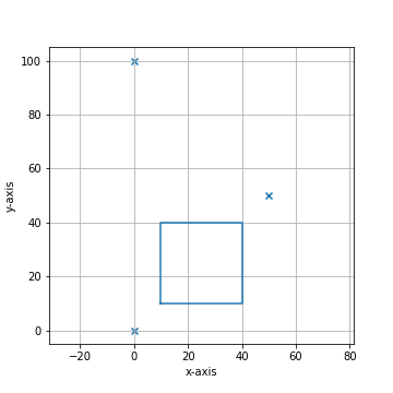
After initiating the coordinate system we can use the rectangle() helper function to create a Shape object with a rectangle with specified size and position.
my_square = tools.rectangle(10, 10, offset=(10,10))
my_first_collection.add_shape(my_square)
my_first_collection.plot(calibration = True)
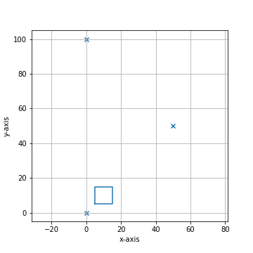
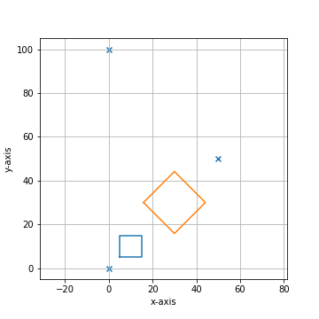
We can further specify an angle of rotation.
my_square = tools.rectangle(20, 20, offset=(30,30), rotation = np.pi/4)
my_first_collection.add_shape(my_square)
my_first_collection.plot(calibration = True)
1.4. Numbers and Letters
The py-lmd tools offer a limited support for numbers and some capital letters. The following glyphs are available: ABCDEFGHI0123456789-_. They were included in the package as they allow for the development of more consistent calibration and sample indexing.In screens with multiple slides, samples can be unambiguously identified from imaged data.
We will first use glyphs() to load single glyphs. The glyphs are included in the py-lmd package as SVG files and are loaded by the svg_to_lmd() into an uncalibrated Collection. This uncalibrated collection is returned and can be joined with a calibrated collection with the join() function.
import numpy as np
from lmd.lib import Collection, Shape
from lmd import tools
calibration = np.array([[0, 0], [0, 100], [50, 50]])
my_first_collection = Collection(calibration_points = calibration)
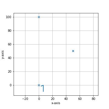
digit_1 = tools.glyph(1)
my_first_collection.join(digit_1)
my_first_collection.plot(calibration = True)
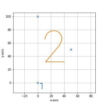
By default glyphs and text have a height of ten units and are located by the top left corner. We can use the offset and multiplier parameters to change the size and position.
digit_2 = tools.glyph(2, offset = (0,80), multiplier = 5)
my_first_collection.join(digit_2)
my_first_collection.plot(calibration = True)
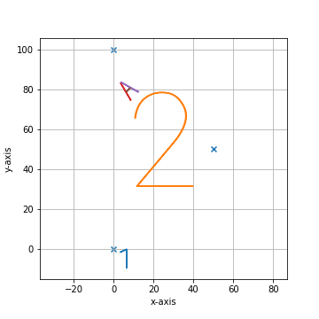
Like with the previous rectangle example we can also use the rotation parameter to set a clockwise rotation.
glyph_A = tools.glyph('A', offset=(0,80), rotation =-np.pi/4)
my_first_collection.join(glyph_A)
my_first_collection.plot(calibration = True)
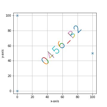
1.5. Text
Next to individual glyphs the text() method can be used to write text with specified position, size and rotation.
import numpy as np
from lmd.lib import Collection, Shape
from lmd import tools

calibration = np.array([[0, 0], [0, 100], [100, 50]])
my_first_collection = Collection(calibration_points = calibration)

identifier_1 = tools.text('0456_B2', offset=np.array([30, 40]), rotation = -np.pi/4)
my_first_collection.join(identifier_1)
my_first_collection.plot(calibration = True)