3.2. Generate cutting XML from exported results from QUPath

The stitched images were loaded into Qupath and specific regions annotaed by hand. calibration points were also selected and labelled with calib1, calib2 and calib3.

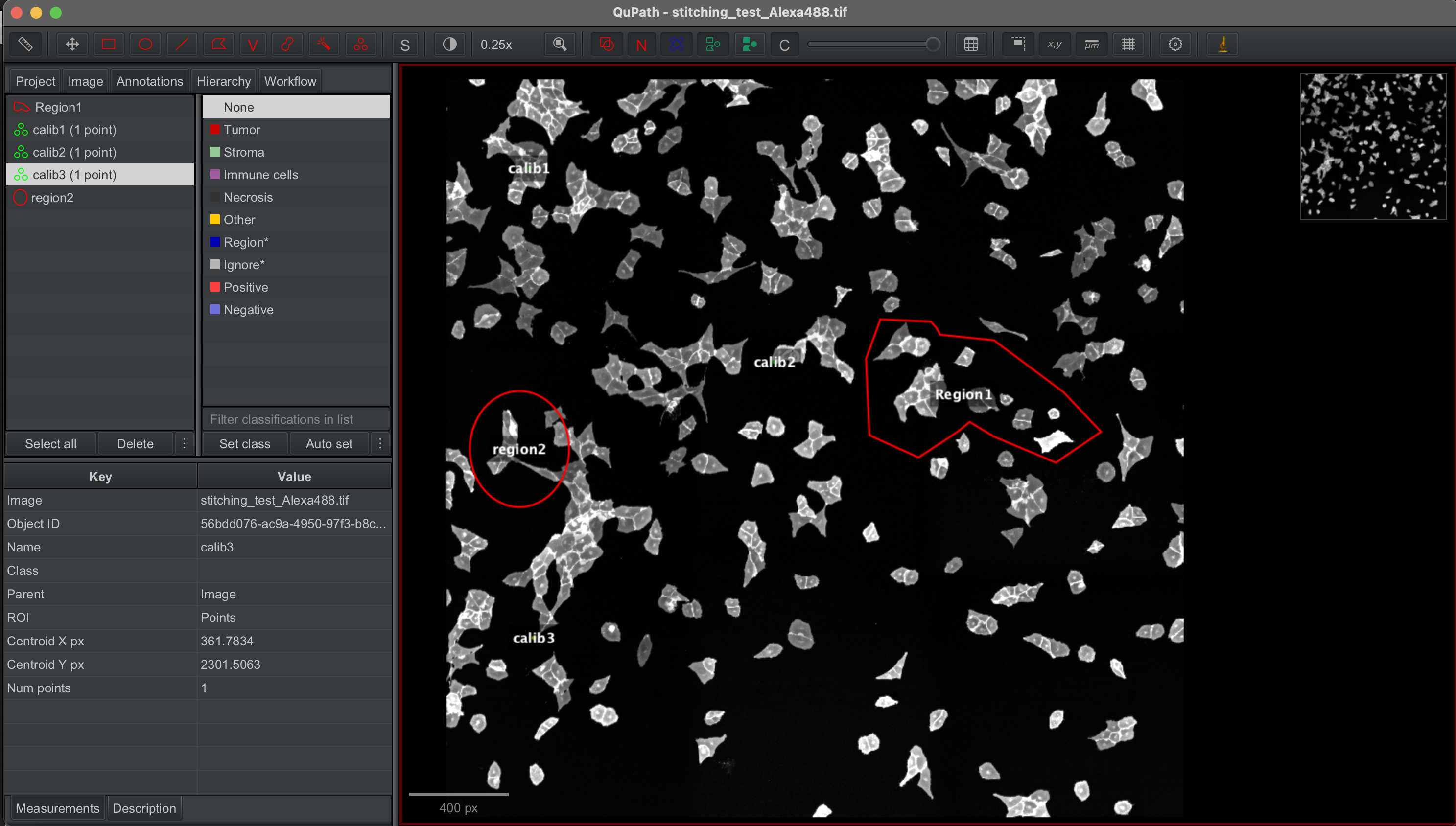
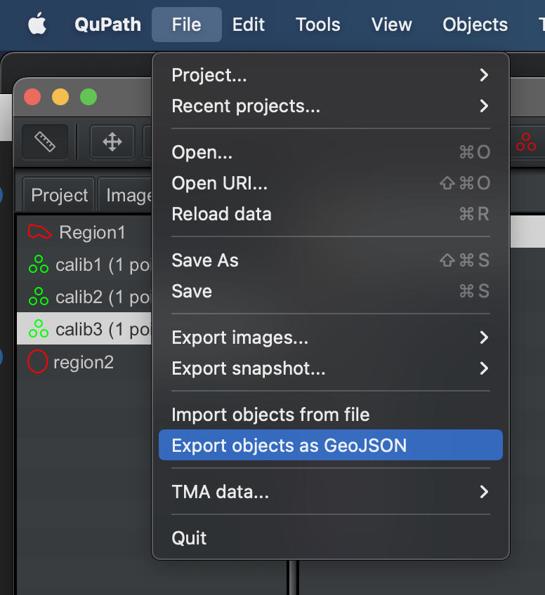
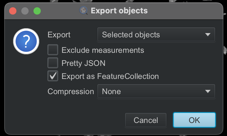
The annotated shapes were then exported to geojson file.

3.2.1. Import libraries and define helper functions

import shapely
import geopandas
import pandas as pd
import numpy as np

from lmd.lib import Collection

def separate_points_polygons(df: geopandas.GeoDataFrame, geometry_column: str = "geometry") -> tuple[geopandas.GeoDataFrame, geopandas.GeoDataFrame]:
    """Split QuPath geopandas dataframe by shape types"""
    points = df[geometry_column].apply(lambda geom: isinstance(geom, shapely.Point))
    polygons = df[geometry_column].apply(lambda geom: isinstance(geom, shapely.Polygon))

    return df.loc[points], df.loc[polygons]

def get_calib_points(list_of_calibpoint_names: str, df: geopandas.GeoDataFrame) -> np.ndarray:
    """Parse selected points into np.array"""

    #Create list of relevant shapes
    pointlist = []
    for point_name in list_of_calibpoint_names:
        pointlist.append(df.loc[df['name'] == point_name, 'geometry'].values[0])

    return np.array([[point.x, point.y] for point in pointlist])

3.2.2. Import GEOjson regions

The geojson dataset is loaded into a dataframe with the following structure:

id	objectType	classification	name	geometry
unique shape id	type of shape (e.g. annotation)	all annotation information from qupath	shape name if given	contains information relevant for shape

The geojson should besides containing individual segemnted shapes contain 3 points annotated as calib1, calib2, calib3 that will be used as calibration points for generating the XML

df = geopandas.read_file("test_data/cellculture_example/annotated_regions_Qupath.geojson")
df

Skipping field color: unsupported OGR type: 1

	id	objectType	name	geometry
0	9287277d-e46f-47e9-aa3f-c540b3318b5e	annotation	region2	POLYGON ((507 1524, 506.6 1539.01, 505.39 1553...
1	ab63cfd3-17d0-4dd3-b8e6-95172dda64de	annotation	Region1	POLYGON ((1789 990, 1730 1153, 1744 1467, 1944...
2	b60d2cf7-963e-42ae-8a2a-69ff289d29db	annotation	calib1	POINT (343.24 368.53)
3	56bdd076-ac9a-4950-97f3-b8c2268ee090	annotation	calib3	POINT (361.78 2301.51)
4	03d9bb6e-16b1-4cd9-9181-86da90fb98bf	annotation	calib2	POINT (1353.77 1165.83)

Annotations and calibration points (shapely.Point objects) and annoatations (shapely.Polygon objects) should be processed separately. Therefore, we will use the previously defined helper function separate_points_polygons to split the dataframe by shape type.

# Separate calibration points (shapely.Points) from annotations (shapely.Polygons)
points, annotations = separate_points_polygons(df)

Let’s inspect the separated geodataframes

points

	id	objectType	name	geometry
2	b60d2cf7-963e-42ae-8a2a-69ff289d29db	annotation	calib1	POINT (343.24 368.53)
3	56bdd076-ac9a-4950-97f3-b8c2268ee090	annotation	calib3	POINT (361.78 2301.51)
4	03d9bb6e-16b1-4cd9-9181-86da90fb98bf	annotation	calib2	POINT (1353.77 1165.83)

annotations

	id	objectType	name	geometry
0	9287277d-e46f-47e9-aa3f-c540b3318b5e	annotation	region2	POLYGON ((507 1524, 506.6 1539.01, 505.39 1553...
1	ab63cfd3-17d0-4dd3-b8e6-95172dda64de	annotation	Region1	POLYGON ((1789 990, 1730 1153, 1744 1467, 1944...

3.2.3. Calibration points

pyLMD expects calibration points as numpy array of the shape (N, 2). We therefore need to extract the coordinates of the calibration points from the points geodataframe. To do so, we will use the second helper function get_calib_points that converts the geometry column of the selected points to a numpy array. Each row in the numpy array represents the coordinates of the calibration points in (x, y) format.

caliblist = get_calib_points(['calib1','calib2','calib3'], points)
caliblist

array([[ 343.24,  368.53],
       [1353.77, 1165.83],
       [ 361.78, 2301.51]])

3.2.4. Generate shape collection

We are now able to convert the annotation dataframe to a collection of shapes. To do so, we initialize an empty pylmd Collection with the previously defined calibration points. We will further define the flip the axes of the points with an orientation_transform as the image coordinates are flipped compared to the microscope coordinates (for a detailed explanation see this tutorial)

annotations

	id	objectType	name	geometry
0	9287277d-e46f-47e9-aa3f-c540b3318b5e	annotation	region2	POLYGON ((507 1524, 506.6 1539.01, 505.39 1553...
1	ab63cfd3-17d0-4dd3-b8e6-95172dda64de	annotation	Region1	POLYGON ((1789 990, 1730 1153, 1744 1467, 1944...

orientation_transform = np.array(
    [
        [1, 0],
        [0, -1]
    ]
)

shape_collection = Collection(
    calibration_points=caliblist,
    orientation_transform=orientation_transform
    )

# Load geopandas into collection class
shape_collection.load_geopandas(annotations, name_column="name")

shape_collection.stats()

===== Collection Stats =====
Number of shapes: 2
Number of vertices: 117
============================
Mean vertices: 58
Min vertices: 16
5% percentile vertices: 20
Median vertices: 58
95% percentile vertices: 97
Max vertices: 101

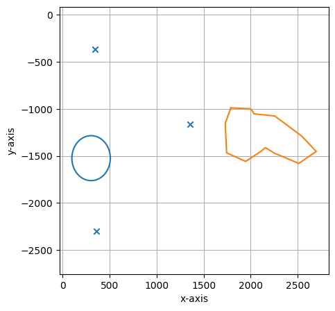
Let’s inspect the loaded annotations and calibration points with the internal plot function:

shape_collection.plot(calibration = True)

3.2.5. Write to XML

You can now write the selection to a Leica-compatible xml file

shape_collection.save("./test_data/cellculture_example/shapes_2.xml")

[ 34324. -36853.]
[ 135377. -116583.]
[  36178. -230151.]