Basic alphapepttools workflow

1. load data and meta data

2. basic minimal preprocessing

3. perform PCA

4. plot PCA embeddings, variance and loadings

import logging
import numpy as np
from pathlib import PureWindowsPath
import pandas as pd

import alphapepttools as at
from alphapepttools.pl.figure import create_figure, label_axes
from alphapepttools.pl.plots import Plots

logging.basicConfig(level=logging.INFO)

Load the data

We download the data from this folder (ca. 2 megabytes)

pg_table_path = at.data.get_data("hela_pg_diann")
metadata_path = at.data.get_data("hela_metadata")

/Users/lucas-diedrich/Documents/Projects/scverse/alphatools/programming/alphatools/docs/notebooks/report.pg_matrix.tsv already exists (1.0532913208007812 MB)
/Users/lucas-diedrich/Documents/Projects/scverse/alphatools/programming/alphatools/docs/notebooks/simple_metadata.csv already exists (0.0013446807861328125 MB)

We can read the data easily with the alphapepttools.io functionalities and match the metadata to the observations

# Read PG table and
# Parse full filepaths to file names (as in metadata file)
# Set uniprot ids as index
adata = at.io.read_pg_table(pg_table_path, search_engine="diann")
adata.obs_names = adata.obs_names.to_series().apply(lambda x: PureWindowsPath(str(x)).stem)
adata.var = adata.var.reset_index(names="protein_names").set_index("uniprot_ids")

# Read metadata
metadata = pd.read_csv(metadata_path, sep=",", index_col="filename")

adata = at.pp.add_metadata(adata=adata, incoming_metadata=metadata, axis=0)
adata

AnnData object with n_obs × n_vars = 18 × 4954
    obs: 'replicate', 'fraction'
    var: 'protein_names', 'genes', 'description'

Basic EDA on a synthetic example dataset:

1. Generate example data

2. Filter for data completeness on sample level

3. Visualize samples as histograms

4. Save data

Filter by data completeness:

Remove features which have more than the allowed fraction of missing values

print("The numeric data in the anndata object:")
display(adata.to_df().head())

print("The sample-level metadata in the anndata object:")
display(adata.obs.head())

print("The feature-level metadata in the anndata object:")
display(adata.var.head())

#  filter out features with more than 25 % missing values
print("Before filtering, the shape of the anndata object: ", adata.shape)
adata = at.pp.filter_data_completeness(adata=adata, max_missing=0.25, action="drop")
print("After filtering, the shape of the anndata object: ", adata.shape)

print("The numeric data in the anndata object:")
display(adata.to_df().head())

print("The sample-level metadata in the anndata object:")
display(adata.obs.head())

print("The feature-level metadata in the anndata object:")
display(adata.var.head())

The numeric data in the anndata object:
The sample-level metadata in the anndata object:
The feature-level metadata in the anndata object:
Before filtering, the shape of the anndata object:  (18, 4954)
After filtering, the shape of the anndata object:  (18, 2831)
The numeric data in the anndata object:
The sample-level metadata in the anndata object:
The feature-level metadata in the anndata object:

uniprot_ids	A0A024R1R8;Q9Y2S6	A0A0B4J2F0	A0A0J9YX75;A0A0J9YXY3;P0DPF7	A0AV96	A0FGR8	A0JLT2	A0PJW6	A1L0T0	A1L390	A1X283	...	Q9Y6N5	Q9Y6N6	Q9Y6N7	Q9Y6N8	Q9Y6R0	Q9Y6V7	Q9Y6W5	Q9Y6X3	Q9Y6X9	Q9Y6Y8
20210131_EXPL4_ViAl_SA_HeLa_Evosep_21min_DIA_120k_15k_1-5_Map2_3K	9506220.0	9930580.0	NaN	6414570.0	29546900.0	NaN	19563300.0	23059400.0	1346120.0	11691800.0	...	39051400.0	172419.0	6796840.0	8998980.0	NaN	NaN	5111880.0	NaN	NaN	7060290.0
20210131_EXPL4_ViAl_SA_HeLa_Evosep_21min_DIA_120k_15k_1-5s_Map1_1K_20210131142601	25866000.0	NaN	NaN	18604800.0	18958500.0	3202770.0	NaN	14090600.0	790375.0	23128600.0	...	10291200.0	NaN	3829290.0	NaN	574729.0	19405500.0	6310680.0	10867000.0	11684000.0	13398300.0
20210131_EXPL4_ViAl_SA_HeLa_Evosep_21min_DIA_120k_15k_1-5s_Map1_3K	10150200.0	11627800.0	NaN	6550420.0	28679800.0	NaN	19387300.0	24248100.0	963907.0	9263040.0	...	38928800.0	NaN	5441930.0	9034600.0	1026870.0	NaN	3963610.0	NaN	NaN	6189950.0
20210131_EXPL4_ViAl_SA_HeLa_Evosep_21min_DIA_120k_15k_1-5s_Map1_6K	14660600.0	8741560.0	NaN	9638120.0	35471700.0	NaN	15716300.0	36269500.0	NaN	11779400.0	...	33905400.0	237138.0	5068170.0	7413300.0	965536.0	NaN	4858220.0	NaN	NaN	6046510.0
20210131_EXPL4_ViAl_SA_HeLa_Evosep_21min_DIA_120k_15k_1-5s_Map1_12K	23477900.0	1497570.0	NaN	16496400.0	27413400.0	NaN	2334540.0	24950500.0	NaN	21687600.0	...	8834620.0	187094.0	3736040.0	4581280.0	1516620.0	NaN	7919380.0	NaN	NaN	9935580.0

5 rows × 4954 columns

	replicate	fraction
20210131_EXPL4_ViAl_SA_HeLa_Evosep_21min_DIA_120k_15k_1-5_Map2_3K	Map2	3K
20210131_EXPL4_ViAl_SA_HeLa_Evosep_21min_DIA_120k_15k_1-5s_Map1_1K_20210131142601	Map1	1K
20210131_EXPL4_ViAl_SA_HeLa_Evosep_21min_DIA_120k_15k_1-5s_Map1_3K	Map1	3K
20210131_EXPL4_ViAl_SA_HeLa_Evosep_21min_DIA_120k_15k_1-5s_Map1_6K	Map1	6K
20210131_EXPL4_ViAl_SA_HeLa_Evosep_21min_DIA_120k_15k_1-5s_Map1_12K	Map1	12K

	protein_names	genes	description
uniprot_ids
A0A024R1R8;Q9Y2S6	TMA7B_HUMAN;TMA7_HUMAN	TMA7;TMA7B	Translation machinery-associated protein 7B
A0A0B4J2F0	PIOS1_HUMAN	PIGBOS1	Protein PIGBOS1
A0A0J9YX75;A0A0J9YXY3;P0DPF7	TVB62_HUMAN;TVB63_HUMAN;TVB69_HUMAN	TRBV6-2;TRBV6-3;TRBV6-9	T cell receptor beta variable 6-9
A0AV96	RBM47_HUMAN	RBM47	RNA-binding protein 47
A0FGR8	ESYT2_HUMAN	ESYT2	Extended synaptotagmin-2

uniprot_ids	A0A024R1R8;Q9Y2S6	A0AV96	A0FGR8	A1L0T0	A1X283	A5PLL7	A5YKK6	A6NCE7;Q9GZQ8	A6NDG6	A6NHR9	...	Q9Y6K5	Q9Y6M0	Q9Y6M1	Q9Y6M4	Q9Y6M5	Q9Y6N7	Q9Y6N8	Q9Y6R0	Q9Y6W5	Q9Y6Y8
20210131_EXPL4_ViAl_SA_HeLa_Evosep_21min_DIA_120k_15k_1-5_Map2_3K	9506220.0	6414570.0	29546900.0	23059400.0	11691800.0	2741150.0	10835800.0	5629360.0	561137.0	3789200.0	...	8955980.0	27799800.0	3070990.0	3151630.0	64329500.0	6796840.0	8998980.0	NaN	5111880.0	7060290.0
20210131_EXPL4_ViAl_SA_HeLa_Evosep_21min_DIA_120k_15k_1-5s_Map1_1K_20210131142601	25866000.0	18604800.0	18958500.0	14090600.0	23128600.0	4624200.0	11243600.0	7728880.0	462468.0	47274600.0	...	9021290.0	18298000.0	NaN	1579620.0	38458300.0	3829290.0	NaN	574729.0	6310680.0	13398300.0
20210131_EXPL4_ViAl_SA_HeLa_Evosep_21min_DIA_120k_15k_1-5s_Map1_3K	10150200.0	6550420.0	28679800.0	24248100.0	9263040.0	3809220.0	10480100.0	7059070.0	700098.0	NaN	...	7307580.0	23668700.0	3084110.0	3130200.0	60378200.0	5441930.0	9034600.0	1026870.0	3963610.0	6189950.0
20210131_EXPL4_ViAl_SA_HeLa_Evosep_21min_DIA_120k_15k_1-5s_Map1_6K	14660600.0	9638120.0	35471700.0	36269500.0	11779400.0	5127720.0	19063600.0	8905940.0	582714.0	NaN	...	12709900.0	39207800.0	6057120.0	3672700.0	56567800.0	5068170.0	7413300.0	965536.0	4858220.0	6046510.0
20210131_EXPL4_ViAl_SA_HeLa_Evosep_21min_DIA_120k_15k_1-5s_Map1_12K	23477900.0	16496400.0	27413400.0	24950500.0	21687600.0	5740560.0	39849800.0	8597510.0	595144.0	3586450.0	...	18124000.0	30144100.0	10509100.0	3353660.0	42608500.0	3736040.0	4581280.0	1516620.0	7919380.0	9935580.0

5 rows × 2831 columns

	replicate	fraction
20210131_EXPL4_ViAl_SA_HeLa_Evosep_21min_DIA_120k_15k_1-5_Map2_3K	Map2	3K
20210131_EXPL4_ViAl_SA_HeLa_Evosep_21min_DIA_120k_15k_1-5s_Map1_1K_20210131142601	Map1	1K
20210131_EXPL4_ViAl_SA_HeLa_Evosep_21min_DIA_120k_15k_1-5s_Map1_3K	Map1	3K
20210131_EXPL4_ViAl_SA_HeLa_Evosep_21min_DIA_120k_15k_1-5s_Map1_6K	Map1	6K
20210131_EXPL4_ViAl_SA_HeLa_Evosep_21min_DIA_120k_15k_1-5s_Map1_12K	Map1	12K

	protein_names	genes	description
uniprot_ids
A0A024R1R8;Q9Y2S6	TMA7B_HUMAN;TMA7_HUMAN	TMA7;TMA7B	Translation machinery-associated protein 7B
A0AV96	RBM47_HUMAN	RBM47	RNA-binding protein 47
A0FGR8	ESYT2_HUMAN	ESYT2	Extended synaptotagmin-2
A1L0T0	HACL2_HUMAN	ILVBL	2-hydroxyacyl-CoA lyase 2
A1X283	SPD2B_HUMAN	SH3PXD2B	SH3 and PX domain-containing protein 2B

Creating new layers prior to preprocessing

This way, we can save the raw data and try different pp steps on the raw data.

# save the raw data before log transformation
adata.layers["raw"] = adata.X.copy()

# log2 transform the data
adata.X = np.log2(adata.X + 1)

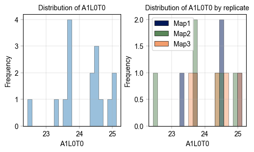
Visualize the distribution of values in different levels of an observational metadata variable

In this example, check the distribution of “gene_1” expression values per cell type.

# Apply the AxisManager to make axes iterable and apply consistent alphapepttools styling.
# Axes can also be accessed directly by indexing the axm object.
fig, axm = create_figure(nrows=1, ncols=2, figsize=(5, 3))

# Plot.histogram handles adata natively. Columns from the data and metadata are accessible
# Focus on the distribution of protein A1L0T0
ax = axm.next()
Plots.histogram(
    data=adata,
    value_column="A1L0T0",
    bins=20,
    legend="auto",
    ax=ax,
    hist_kwargs={"alpha": 0.5, "histtype": "stepfilled", "linewidth": 0.5, "edgecolor": "black"},
)
label_axes(ax, "A1L0T0", "Frequency", "Distribution of A1L0T0")

# Focus on the distribution of protein A1L0T0 in the different replicates
ax = axm.next()
Plots.histogram(
    data=adata,
    value_column="A1L0T0",
    color_map_column="replicate",
    bins=20,
    legend="auto",
    ax=ax,
    hist_kwargs={"alpha": 0.5, "histtype": "stepfilled", "linewidth": 0.5, "edgecolor": "black"},
)
label_axes(ax, "A1L0T0", "Frequency", "Distribution of A1L0T0 by replicate")

# # save figure
# save_figure(
#     fig=fig,
#     filename="sample_histogram.png",
#     output_dir=output_directory,
#     dpi=300,
#     transparent=False,
# )

Running PCA

Before running PCA, we need to filter out NaN values. PCA can not be computed on matrices with missing values. Therefore, prior to PCA, we will create a list of ‘core proteins’ of proteins detected in all observations, save it in the feature meta data frame (adata.var)

# add a new column to the adata.var object with the name "is_core" to indicate whether the feature is part of the core proteome
adata = at.pp.filter_data_completeness(adata, max_missing=0, action="flag", var_colname="is_core")

# view hoe many features are part of the core proteome
print("The number of features in the core proteome:")
print(adata.var["is_core"].value_counts())

The number of features in the core proteome:
is_core
True     1806
False    1025
Name: count, dtype: int64

Now we can run PCA, specifying the adata.var column that filters the proteins by 100% completeness:

# this function is now implemented on sample level (PCA of the observations).
at.tl.pca(adata, meta_data_mask_column_name="is_core", n_comps=10)

# view the PCA results
print("The dimensions of PC coordinates in the adata.obsm are (n_obs x n_comp):")
print(adata.obsm["X_pca_obs"].shape)
print("The PCA loadings in the adata.varm are (n_var x n_comp):")
print(adata.varm["PCs_obs"].shape)
print("Ratio of explained variance (n_comp):")
print(adata.uns["variance_pca_obs"]["variance_ratio"])
print("The explained variance (n_comp):")
print(adata.uns["variance_pca_obs"]["variance"])

The dimensions of PC coordinates in the adata.obsm are (n_obs x n_comp):
(18, 10)
The PCA loadings in the adata.varm are (n_var x n_comp):
(2831, 10)
Ratio of explained variance (n_comp):
[0.56593504 0.33056594 0.06844902 0.01339105 0.00388991 0.00288049
 0.0023081  0.00220095 0.00194543 0.0017315 ]
The explained variance (n_comp):
[1009.50632405  589.65850994  122.09831939   23.88675892    6.93875425
    5.13817412    4.11715411    3.92601867    3.47022027    3.08861607]

In addition to running PCA to get a dimentional reduction of the observations (samples), we can also perform PCA on the features (proteins).

# Now run PCA on the protein space to get their projection in the PCA space.
at.tl.pca(adata, meta_data_mask_column_name="is_core", n_comps=10, dim_space="var")

# view the PCA results for features
print("----- PCA ON FEATURES -----")
print("The dimensions of PC coordinates in the adata.varm are (n_obs x n_comp):")
print(adata.varm["X_pca_var"].shape)
print("The PCA loadings of the samples in the adata.obsm are (n_var x n_comp):")
print(adata.obsm["PCs_var"].shape)
print("Ratio of explained variance (n_comp):")
print(adata.uns["variance_pca_var"]["variance_ratio"])
print("The explained variance (n_comp):")
print(adata.uns["variance_pca_var"]["variance"])

----- PCA ON FEATURES -----
The dimensions of PC coordinates in the adata.varm are (n_obs x n_comp):
(2831, 10)
The PCA loadings of the samples in the adata.obsm are (n_var x n_comp):
(18, 10)
Ratio of explained variance (n_comp):
[8.07567317e-01 1.13818512e-01 6.33157115e-02 8.74927065e-03
 2.21018860e-03 7.89962453e-04 5.76627224e-04 4.64255895e-04
 4.48561680e-04 3.63473757e-04]
The explained variance (n_comp):
[6.64865141e+01 9.37060716e+00 5.21274308e+00 7.20322002e-01
 1.81963451e-01 6.50371166e-02 4.74733601e-02 3.82218986e-02
 3.69298036e-02 2.99245680e-02]

Plot PCA results

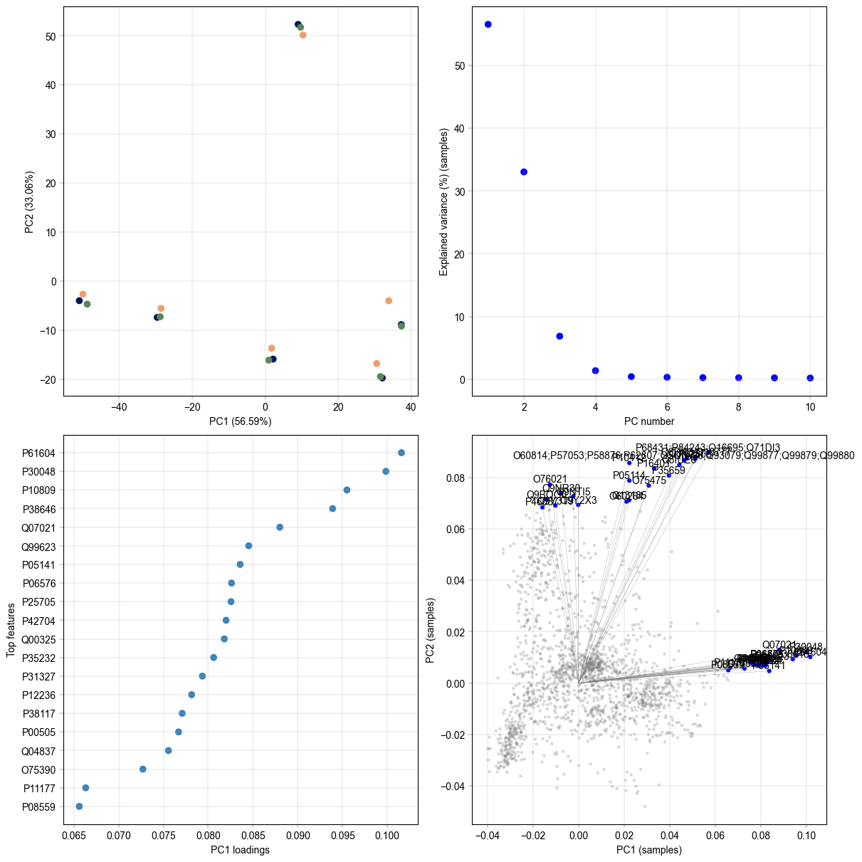
We can plot the PCA results on a 2D projection, look at the explained var in each PC using the scree plot, and plot the loadings od the PCs, either per PC or a scatter of 2 PCs, to understand their ‘drivers’.

fig, axm = create_figure(2, 2, figsize=(12, 12))

ax = axm.next()
# PCA plot colored by replicate
Plots.plot_pca(
    data=adata,
    ax=ax,
    x_column=1,
    y_column=2,
    label=False,
    label_column=None,
    embeddings_name=None,
    color_map_column="replicate",
)

# scree plot to show the explained variance by each PC
ax = axm.next()
Plots.scree_plot(adata=adata, ax=ax, n_pcs=50)

# top loadings of the first PC
ax = axm.next()
Plots.plot_pca_loadings(
    data=adata,
    ax=ax,
    dim=1,
    nfeatures=20,
)

# 2d loading plot with highlighted top 20 loadings
ax = axm.next()
Plots.plot_pca_loadings_2d(
    data=adata,
    ax=ax,
    pc_x=1,
    pc_y=2,
    nfeatures=20,
    add_labels=True,
    add_lines=True,
    scatter_kwargs=None,
)

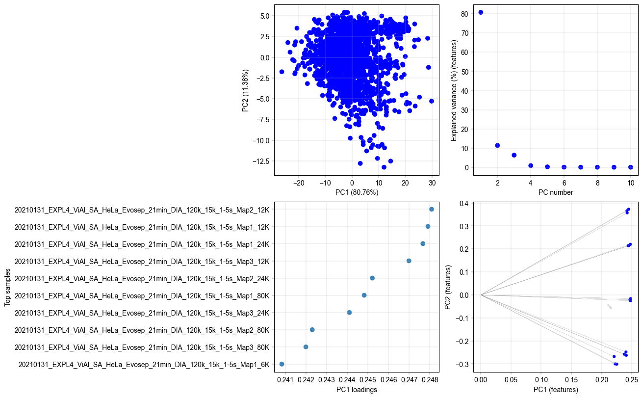
Plot PCA results for feature PCA

Just like the PCA on the samples, we can plot the same plots for the results of PCA calculated on the features.

# now produce the PCAs plot for the features
fig, axm = create_figure(2, 2, figsize=(13, 8))

ax = axm.next()
Plots.plot_pca(
    data=adata,
    ax=ax,
    x_column=1,
    y_column=2,
    dim_space="var",
    label=False,
    label_column=None,
    embeddings_name=None,
)

ax = axm.next()
Plots.scree_plot(adata=adata, ax=ax, n_pcs=50, dim_space="var")

ax = axm.next()
Plots.plot_pca_loadings(data=adata, ax=ax, dim=1, nfeatures=10, dim_space="var")

ax = axm.next()
Plots.plot_pca_loadings_2d(
    data=adata,
    ax=ax,
    pc_x=1,
    pc_y=2,
    nfeatures=10,
    add_labels=False,
    add_lines=True,
    scatter_kwargs=None,
    dim_space="var",
)

UMAP Visualization with Scanpy

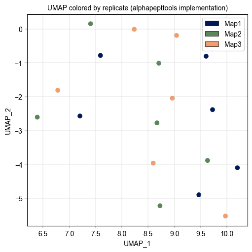
To explore and visualize the high-dimensional proteomics data, we use UMAP (Uniform Manifold Approximation and Projection) as implemented in Scanpy. UMAP projects complex, high-dimensional feature spaces into a lower-dimensional space (typically 2D) while preserving the local and global structure of the data. This allows us to identify clusters, relationships, and potential outliers in the proteomic profiles at a glance.

In this notebook, Scanpy’s sc.pp.neighbors() and sc.tl.umap() functions are applied to the processed data matrix to compute a nearest-neighbor graph and then generate UMAP coordinates. We will use the sample PCA matrix for neighbor calculations. The resulting UMAP embedding provides an intuitive visualization of sample similarity and grouping based on proteomic features, complementing downstream analyses such as clustering or differential expression.

import scanpy as sc

sc.pp.neighbors(adata, n_neighbors=10, use_rep="X_pca_obs")  # use the PCA results on samples
sc.tl.umap(adata)

# location of the umap coordinates in the adata.obsm
print("The UMAP coordinates in the adata.obsm are in adata.obsm['X_umap'] with shape: ", adata.obsm["X_umap"].shape)
print(adata.obsm["X_umap"])

The UMAP coordinates in the adata.obsm are in adata.obsm['X_umap'] with shape:  (18, 2)
[[23.248234   -1.2672713 ]
 [22.80575    -0.08841316]
 [23.620588   -0.6427061 ]
 [24.165075   -1.5532923 ]
 [24.523983   -0.21402165]
 [25.940697   -1.1079656 ]
 [26.18492     0.780279  ]
 [23.35512     0.42271757]
 [24.21046    -2.5432775 ]
 [24.973011   -0.9202459 ]
 [26.795399   -0.45468578]
 [26.0829     -0.18279085]
 [24.299662    0.8317656 ]
 [22.442497   -1.0312376 ]
 [25.063112   -2.0696015 ]
 [23.163307   -2.339625  ]
 [26.056355   -1.930257  ]
 [25.28021     0.37642172]]

Plot UMAP

We can either plot the UMAP results using scanpy’s plotting function, or we can use alphapepttools plotting function, with adding the umap coordinates directly to the obs df.

# scanpy's plotting function
sc.pl.umap(adata, color="replicate", size=100)  # the size is usually much smaller

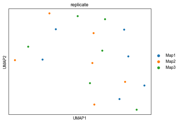
Another option is to copy the coordinates into the adata.obs data frame, to plot in using scatter function in alphapepttools package

adata.obs["UMAP1"] = adata.obsm["X_umap"][:, 0]
adata.obs["UMAP2"] = adata.obsm["X_umap"][:, 1]

fig, axm = create_figure(1, 1, figsize=(5, 5))
ax = axm.next()
Plots.scatter(adata, x_column="UMAP1", y_column="UMAP2", color_map_column="replicate", ax=ax, legend="auto")

label_axes(
    ax=ax,
    xlabel="UMAP_1",
    ylabel="UMAP_2",
    title="UMAP colored by replicate (alphapepttools implementation)",
)