Example of PELSA differential expression with alphapepttools

An example dataset: The original PELSA publication

PELSA [1] is a novel method to investigate protein-ligand interactions through limited proteolysis. Cell lysate is treated with a short pulse of trypsin at extremely high (1:2) enzyme - substrate ratio, which allows for the digestion of surface exposed peptides. If a ligand (such as a small molecule binder) is bound to the protein surface, it stablizes the surrounding protein region and digestion is momentarily slowed. When compared against a control without the ligand, the PELSA-stabilized peptides appear downregulated. We replicate the original publication’s analysis of Staurosporine, a pan-kinase binder, and visualize the regulation of kinase targets.

[1]: Li, Kejia, et al. “A peptide-centric local stability assay enables proteome-scale identification of the protein targets and binding regions of diverse ligands.” Nature Methods 22.2 (2025): 278-282.

import tempfile
import pandas as pd
import numpy as np
import logging
import alphapepttools as at  # import io, pp, pl, tl  # input/output, preprocessing, plotting and tools modules
from matplotlib.patches import Rectangle

logger = logging.getLogger(__name__)

Preparing the dataset using alphapepttools loaders and AnnData factory.

After downloading the relevant files from the study’s PRIDE-repository (https://www.ebi.ac.uk/pride/archive/projects/PXD034606):

• LKJ_20211007_480_Hela_stau_0uM_1.raw

• LKJ_20211007_480_Hela_stau_0uM_2.raw

• LKJ_20211007_480_Hela_stau_0uM_3.raw

• LKJ_20211007_480_Hela_stau_0uM_4.raw

• LKJ_20211007_480_Hela_stau_20uM_1.raw

• LKJ_20211007_480_Hela_stau_20uM_2.raw

• LKJ_20211007_480_Hela_stau_20uM_3.raw

• LKJ_20211007_480_Hela_stau_20uM_4.raw

And processing them with DIANN 2.1.0, the report.parquet file was saved in our datashare alongside sample metadata. We have to extract protein-level intensities and precursor-level intensities from this dataset using the alphapepttools.io.AnnDataFactory class. The resulting AnnData object contains protein-group or precursor quantities and any number of feature-metadata columns (for example, protein groups may have genes as secondary annotation, precursors may have protein groups and genes as secondary annotation).

# Download the data using the alphapepttools data module
report_path = at.data.get_data("pelsa_report_diann", output_dir=tempfile.mkdtemp())
sample_metadata_path = at.data.get_data("pelsa_metadata", output_dir=tempfile.mkdtemp())

# Get the full report
full_report = pd.read_parquet(report_path)

# AnnDataFactory instance containing protein level data
adata_protein = at.io.read_psm_table(
    file_paths=report_path,
    search_engine="diann",
    level="proteins",
    var_columns=["genes"],
)

# AnnDataFactory instance containing gene level data
adata_gene = at.io.read_psm_table(
    file_paths=report_path,
    search_engine="diann",
    level="genes",
)

# AnnDataFactory instance containing precursor level data
adata_precursor = at.io.read_psm_table(
    file_paths=report_path,
    search_engine="diann",
    intensity_column="Precursor.Normalised",
    feature_id_column="Precursor.Id",
    sample_id_column="Run",
    var_columns=["proteins", "genes", "sequence"],
)

/var/folders/2l/hhd_z4hx3070zw8rlj4c3l940000gn/T/tmp5j3sii7k/report.parquet does not yet exist
/var/folders/2l/hhd_z4hx3070zw8rlj4c3l940000gn/T/tmp5j3sii7k/report.parquet successfully downloaded (70.8467435836792 MB)
/var/folders/2l/hhd_z4hx3070zw8rlj4c3l940000gn/T/tmpr1853dya/iteration_L_literature_reprocessing_PELSA_samplemap.csv does not yet exist
/var/folders/2l/hhd_z4hx3070zw8rlj4c3l940000gn/T/tmpr1853dya/iteration_L_literature_reprocessing_PELSA_samplemap.csv successfully downloaded (0.000179290771484375 MB)

We focus on Protein Groups and Precursors, and use pp.add_metadata() to merge the metadata into our AnnData instances

# Transfer the run names to the sample metadata to account for lack of rawfile names in the metadata
sample_metadata = pd.read_csv(sample_metadata_path)
sample_metadata["sample"] = sample_metadata["plate"] + "_" + sample_metadata["running_count"].astype(str)

run_name_map = {"_".join(k.split("_")[-2:]): k for k in adata_protein.obs_names}
sample_metadata.index = sample_metadata["sample"].map(run_name_map)

# Add the metadata to all AnnData instances
adata_protein = at.pp.add_metadata(adata_protein, sample_metadata, axis=0)
adata_precursor = at.pp.add_metadata(adata_precursor, sample_metadata, axis=0)

We log2-transform our data, but keep the untransformed values in a separate layer

adata_protein.layers["raw"] = adata_protein.X.copy()
adata_precursor.layers["raw"] = adata_precursor.X.copy()

at.pp.nanlog(adata_protein)
at.pp.nanlog(adata_precursor)

# Inspect the log2-transformed values:
display(adata_protein.to_df().iloc[:5, :5])

# Raw values:
display(adata_protein.to_df(layer="raw").iloc[:5, :5])

proteins	A0A096LP55;P07919	A0A0B4J2F0	A0A1B0GUY1	A0A3B3IS91	A0A3B3IU46;Q9BTL3
raw_name
LKJ_20211007_480_Hela_stau_0uM_1	21.790016	23.018673	24.692411	17.029541	23.745449
LKJ_20211007_480_Hela_stau_0uM_2	21.902254	23.051476	24.746101	17.110256	23.861660
LKJ_20211007_480_Hela_stau_0uM_3	21.277990	23.003662	24.555399	17.807335	23.645226
LKJ_20211007_480_Hela_stau_0uM_4	21.540596	23.048594	24.787121	16.149979	23.457727
LKJ_20211007_480_Hela_stau_20uM_1	21.918283	23.059902	24.633326	NaN	23.821888

proteins	A0A096LP55;P07919	A0A0B4J2F0	A0A1B0GUY1	A0A3B3IS91	A0A3B3IU46;Q9BTL3
raw_name
LKJ_20211007_480_Hela_stau_0uM_1	3626171.50	8497893.0	27111686.0	133783.515625	14063468.0
LKJ_20211007_480_Hela_stau_0uM_2	3919543.50	8693320.0	28139656.0	141481.781250	15243168.0
LKJ_20211007_480_Hela_stau_0uM_3	2542808.25	8409926.0	24655366.0	229372.937500	13119653.0
LKJ_20211007_480_Hela_stau_0uM_4	3050461.00	8675965.0	28951204.0	72715.656250	11520718.0
LKJ_20211007_480_Hela_stau_20uM_1	3963336.50	8744247.0	26023742.0	NaN	14828694.0

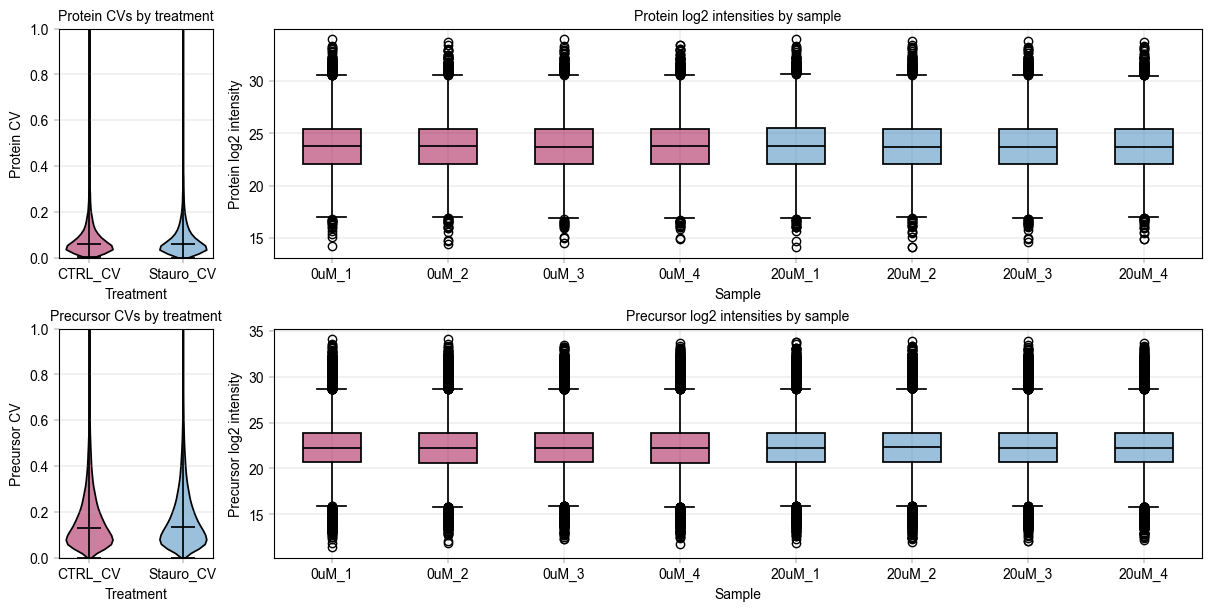
Perform basic EDA on protein and precursor data

Starting with a panel for feature counts and CVs in each sample

# Small custom function to generate CVs
# In the future, this could become an alphapepttools core functionality
import anndata as ad


def make_group_cvs(
    adata: ad.AnnData,
    group_column: str,
) -> None:
    """Calculate CVs for each group in group_columns and store them in adata.var"""
    levels = adata.obs[group_column].unique()
    for level in levels:
        group_adata = at.pp.filter_by_metadata(adata, {group_column: level}, axis=0)
        stds = group_adata.to_df(layer="raw").std(axis=0)
        means = group_adata.to_df(layer="raw").mean(axis=0)
        adata.var[f"{level}_CV"] = stds / means


# Calculate CVs for the different groups in the condition column
make_group_cvs(adata_protein, "treatment")
make_group_cvs(adata_precursor, "treatment")

We use alphapepttools’ plotting syntax to generate a stylized panel with violin plots for sample group feature CVs, and to assess the median intensity of all features across samples.

fig, axm = at.pl.create_figure(2, 2, figsize=(12, 6), gridspec_kwargs={"width_ratios": [0.5, 3]})

# Define color dictionary for the different treatments
color_dict = {
    "CTRL": at.pl.BaseColors.get("red"),
    "Stauro": at.pl.BaseColors.get("blue"),
}

# Map the sample names to their respective colors based on treatment
sample_color_dict = {
    sample: color_dict[treatment]
    for sample, treatment in zip(adata_protein.obs_names, adata_protein.obs["treatment"], strict=False)
}

# Iterative plotting
plot_data = {
    "protein": adata_protein,
    "precursor": adata_precursor,
}
for readout, adata in plot_data.items():
    # start with the CV plots
    ax = axm.next()
    at.pl.Plots.violinplot(
        ax=ax,
        data=adata.T,
        direct_columns=["CTRL_CV", "Stauro_CV"],
        color_dict={f"{k}_CV": v for k, v in color_dict.items()},
    )
    ax.set_ylim(0, 1)

    at.pl.label_axes(
        ax=ax,
        xlabel="Treatment",
        ylabel=f"{readout.capitalize()} CV",
        title=f"{readout.capitalize()} CVs by treatment",
    )

    # Then do the log2 abundance plots
    ax = axm.next()
    at.pl.Plots.boxplot(
        ax=ax,
        data=adata.T,
        direct_columns=adata.obs_names.tolist(),
        color_dict=sample_color_dict,
    )

    # process x ticks to fit the plot better
    xtick_labels = [item.get_text() for item in ax.get_xticklabels()]  # Get xtick labels directly from axes
    xtick_labels = [
        "_".join(x.split("_")[-2:]) for x in xtick_labels
    ]  # Shorten the xtick labels to make them more readable
    _ = ax.set_xticklabels(xtick_labels)  # Set the new xtick labels

    at.pl.label_axes(
        ax=ax,
        xlabel="Sample",
        ylabel=f"{readout.capitalize()} log2 intensity",
        title=f"{readout.capitalize()} log2 intensities by sample",
    )

    # save figure
    at.pl.save_figure(
        fig=fig,  # Note that here we're using the whole figure to whose axes we added our plots
        filename="pelsa_quantities_overview.svg",
        output_dir="./example_outputs",
    )

PELSA analysis depends on differential expression

Peptides from the stablized protein regions are expected to appear downregulated. We perform comparative differential expression analysis:

• On the one hand, we evaluate “vanilla” independent two-sample t-test.

• On the other, we employ alphapepttools’ wrapper of AlphaQuant [1], a differential expression method specially adapted for mass-spectrometry proteomics data.

• Additionally, we examine a Python-implementation of the popular Limma package’s Empirical Bayes moderated ttest, which is more sophisticated than a simple ttest but considerably faster and more lightweight than alphaquant.

We want to retain the original AnnData object’s feature-level metadata in our differential expression results, which can be accomplished by joining the var object to the results.

[1]: Ammar, Constantin, et al. “Tree-based quantification infers proteoform regulation in bottom-up proteomics data.” bioRxiv (2025): 2025-03.

comparison = ("Stauro", "CTRL")

# Vanilla ttest on peptide data
ttest_peptide_results = at.tl.diff_exp_ttest(
    adata=adata_precursor,
    between_column="treatment",
    comparison=comparison,
    min_valid_values=3,
    equal_var=False,
)
ttest_peptide_results = ttest_peptide_results.join(adata_precursor.var, how="left")

Comparing groups: Stauro vs CTRL

# Run Limma Empirical Bayes moderated ttest on peptides: alphapepttools inmoose
ebayes_peptide_results = at.tl.diff_exp_ebayes(
    adata=adata_precursor,
    between_column="treatment",
    comparison=comparison,
)[1]
ebayes_peptide_results = ebayes_peptide_results.join(adata_precursor.var, how="left")

# AlphaQuant ttest on full search engine output (takes approx. 3-4 minutes on a M2 MacBook Pro. Set "REPROCESS" flag to True to re-run, otherwise cached data will be used)
REPROCESS = False

if REPROCESS:
    comparison_key, alphaquant_results = at.tl.diff_exp_alphaquant(
        adata=adata_precursor,
        report=full_report,
        between_column="treatment",
        comparison=comparison,
        valid_values_filter_mode="either",
        min_valid_values=3,
        plots="hide",
    )
    alphaquant_peptide_results = alphaquant_results["peptide"]
    alphaquant_peptide_results.to_pickle("./example_data/notebook_04_alphaquant_peptide_results.pkl")
else:
    logger.info(" --> Using cached AlphaQuant results")
    alphaquant_peptide_results = pd.read_pickle("./example_data/notebook_04_alphaquant_peptide_results.pkl")

Alphaquant results are saved into a dictionary based on the quantification level:

• results

  • protein level results

  • proteoform level results

  • peptide level results

We can use alphapepttools functionality to construct a volcanoplot function

alphapepttools does not have a dedicated volcanoplotting function. However, it is straightforward to assemble one from the tools already implemented. In its basic form, a volcanoplot consists of:

• figure canvas (pl.create_figure())

• scatterplot (pl.Plots.scatter())

• lines (pl.add_lines())

• labels (pl.label_plot())

• axis labels (pl.label_axes())

In the publication, peptides are aggregated into proteins in a nonstandard way: For each protein, the peptide with the highest significance is assigned its protein ID. This is how a dataset of peptides is converted into a dataset of proteins. We perform the same aggregation in our preprocessing.

ebayes_peptide_results

	condition_pair	protein	log2fc	p_value	-log10(p_value)	fdr	-log10(fdr)	method	max_level_1_samples	max_level_2_samples	stat	B	AveExpr	proteins	genes	sequence	CTRL_CV	Stauro_CV
(UniMod:1)AAAAAAAGDSDSWDADAFSVEDPVR3	Stauro_VS_CTRL	(UniMod:1)AAAAAAAGDSDSWDADAFSVEDPVR3	-0.779220	0.009479	2.023230	0.560184	0.251669	limma_ebayes_inmoose	4	4	-3.326301	-2.842216	24.208256	O75822	EIF3J	AAAAAAAGDSDSWDADAFSVEDPVR	0.348759	0.168788
(UniMod:1)AAAAAAAGDSDSWDADAFSVEDPVRK3	Stauro_VS_CTRL	(UniMod:1)AAAAAAAGDSDSWDADAFSVEDPVRK3	-0.163618	0.465420	0.332155	0.960454	0.017523	limma_ebayes_inmoose	4	4	-0.763940	-6.411124	20.255520	O75822	EIF3J	AAAAAAAGDSDSWDADAFSVEDPVRK	0.255562	0.243771
(UniMod:1)AAAAAAAPSGGGGGGEEERLEEK3	Stauro_VS_CTRL	(UniMod:1)AAAAAAAPSGGGGGGEEERLEEK3	0.131008	0.226355	0.645211	0.933111	0.030067	limma_ebayes_inmoose	4	4	1.303456	-5.869777	20.313845	P51608-2	MECP2	AAAAAAAPSGGGGGGEEERLEEK	0.116230	0.060557
(UniMod:1)AAAAAAGAASGLPGPVAQGLK3	Stauro_VS_CTRL	(UniMod:1)AAAAAAGAASGLPGPVAQGLK3	-0.001897	0.985646	0.006279	0.999811	0.000082	limma_ebayes_inmoose	4	4	-0.018523	-6.721547	22.979843	Q96P70	IPO9	AAAAAAGAASGLPGPVAQGLK	0.064267	0.109800
(UniMod:1)AAAAAAGEAR2	Stauro_VS_CTRL	(UniMod:1)AAAAAAGEAR2	0.120329	0.590239	0.228972	0.972137	0.012272	limma_ebayes_inmoose	4	4	0.559355	-6.552634	21.665287	P09417;P09417-2	QDPR	AAAAAAGEAR	0.314222	0.103197
...	...	...	...	...	...	...	...	...	...	...	...	...	...	...	...	...	...	...
YYVTIIDAPGHRDFIK3	Stauro_VS_CTRL	YYVTIIDAPGHRDFIK3	0.296327	0.030165	1.520504	0.743737	0.128581	limma_ebayes_inmoose	4	4	2.594342	-4.001476	21.721304	P68104	EEF1A1	YYVTIIDAPGHRDFIK	0.093635	0.124795
YYVTIIDAPGHRDFIK4	Stauro_VS_CTRL	YYVTIIDAPGHRDFIK4	0.047830	0.727330	0.138268	0.984444	0.006809	limma_ebayes_inmoose	4	4	0.360320	-6.650818	24.960939	P68104	EEF1A1	YYVTIIDAPGHRDFIK	0.138696	0.122280
YYYQLNSK2	Stauro_VS_CTRL	YYYQLNSK2	0.039897	0.719846	0.142760	0.983339	0.007297	limma_ebayes_inmoose	4	4	0.370719	-6.646698	23.494913	O00257	CBX4	YYYQLNSK	0.115134	0.081185
YYYSDNFFDGQR2	Stauro_VS_CTRL	YYYSDNFFDGQR2	-0.014498	0.928952	0.032007	0.997290	0.001179	limma_ebayes_inmoose	4	4	-0.091820	-6.717097	22.013996	Q9H4B6	SAV1	YYYSDNFFDGQR	0.152211	0.177059
YYYVQNVYTPVDEHVYPDHR3	Stauro_VS_CTRL	YYYVQNVYTPVDEHVYPDHR3	0.020215	0.833917	0.078877	0.990898	0.003971	limma_ebayes_inmoose	4	4	0.216166	-6.696086	23.499073	Q86TG7-4	PEG10	YYYVQNVYTPVDEHVYPDHR	0.040443	0.107898

68670 rows × 18 columns

def top_peptides_to_proteins(
    ttest_df: pd.DataFrame,
    y_score_column: str = "-log10(p_value)",
    id_column: str = "protein",
) -> pd.DataFrame:
    """Convert peptide level t-test results to protein level by taking the top peptide per protein."""
    ttest_df = ttest_df.copy()
    return ttest_df.sort_values(y_score_column, ascending=False).groupby(id_column).first().reset_index()


aq_protein_table = top_peptides_to_proteins(alphaquant_peptide_results, id_column="protein")
eb_protein_table = top_peptides_to_proteins(ebayes_peptide_results, id_column="genes")
tt_protein_table = top_peptides_to_proteins(ttest_peptide_results, id_column="genes")

Additionally, we have to annotate all kinases in the data in order to visualize them and perform kinase enrichment scoring. To do this, we load a table from Gerard et al. [1] (http://www.kinhub.org/kinases.html) and transfer the annotations to our data.

[1]: Manning, Gerard, et al. “The protein kinase complement of the human genome.” Science 298.5600 (2002): 1912-1934.

def annotate_kinases(
    ttest_df: pd.DataFrame,
    kinase_table_path: str,
    gene_id_column: str = "gene",
) -> list:
    """Assign str value for kinase/no kinase based on publication data:

    Manning, Gerard, et al. "The protein kinase complement of the human genome." Science 298.5600 (2002): 1912-1934.,
    table from: http://www.kinhub.org/kinases.html

    """
    ttest_df = ttest_df.copy()
    kinase_table = pd.read_excel(kinase_table_path)
    kinase_list = kinase_table["HGNC Name"].tolist()
    kinase_dict = dict(zip(kinase_list, ["kinase"] * len(kinase_list), strict=False))

    ttest_df["kinase_status"] = ttest_df[gene_id_column].map(kinase_dict).fillna("other")
    return ttest_df


# Download the kinase table using the alphapepttools data module
kinase_path = at.data.get_data("kinase_table")

tt_protein_table = annotate_kinases(tt_protein_table, kinase_path, "genes")
eb_protein_table = annotate_kinases(eb_protein_table, kinase_path, "genes")
aq_protein_table = annotate_kinases(aq_protein_table, kinase_path, "protein")

/Users/vincenthbrennsteiner/Documents/mann_labs/_git_repositories/alphapepttools/docs/notebooks/kinome_table.xlsx already exists (0.06418609619140625 MB)

The main readout is a custom Kinase Enrichment Score:

In the main publication [1] and its follow-up [2], a kinase score is implemented to assess the sensitivity and specificity of the assay. This score derives from the fact that, in the ideal case we should only see kinase peptides downregulated. In practice, there are off-targets, i.e. peptides/proteins that appear as downregulated even though they are not kinases. The score is the ratio of downregulated (log2fc < 0) kinases/non-kinases at 80 % specificity when ranking by -log10(p_value).

Imagine a boundary moving down from the highest point in the left half of the volcanoplot. Each time it passes a point, we count if the point is a kinase or a non-kinase. When the ratio of passed kinases / passed non-kinases becomes smaller than 0.8 we state that 80 % specificity is reached. However many kinases we have up to this point is our score.

[1]: Li, Kejia, et al. “A peptide-centric local stability assay to unveil protein targets of diverse ligands.” bioRxiv (2023): 2023-10.

[2]: Li, Kejia, et al. “High-throughput peptide-centric local stability assay extends protein-ligand identification to membrane proteins, tissues, and bacteria.” bioRxiv (2025): 2025-04.

def kinase_score(
    ttest_df: pd.DataFrame,
    id_col: str,
    score_column: str = "-log10(p_value)",
    max_candidates: int = 500,
    threshold: float = 0.8,
) -> dict | None:
    """Perform kinase scoring analysis per HT-Pelsa.

    1. Sort peptides by -log10(significance) (score_column) descending
    2. Consider only regulated peptides, i.e. log2fc < 0
    3. Iterate through ranks, calculating the cumulative kinase fraction
         (number of kinases / total number of peptides)
    4. Stop when kinase fraction drops below min_kinase_pct or max_candidates is reached

    """
    ttest_df = ttest_df.copy()
    print(
        f"Total unique kinases in the dataset: {ttest_df.loc[ttest_df['kinase_status'] == 'kinase', id_col].nunique()}"
    )

    # Restrict to downregulated peptides
    ttest_df = ttest_df[ttest_df["log2fc"] < 0]
    print(
        f"Total unique kinases in the downregulated dataset: {ttest_df.loc[ttest_df['kinase_status'] == 'kinase', id_col].nunique()}"
    )

    # Rank peptides by score
    ttest_df = ttest_df.sort_values(score_column, ascending=False).reset_index(drop=True)
    ttest_df["rank"] = ttest_df.index + 1

    # Iterate through ranks and record the kinase fraction
    def _kinase_fraction(df: pd.DataFrame) -> float:
        kinase_count = df[df["kinase_status"] == "kinase"].shape[0]
        total_count = df.shape[0]
        return kinase_count / total_count if total_count > 0 else np.nan

    kinase_fractions = []
    for n in range(1, len(ttest_df) + 1):
        subset = ttest_df.head(n)
        kinase_fraction = _kinase_fraction(subset)
        score_threshold = subset[score_column].iloc[-1]
        kinase_fractions.append(
            {
                "rank": n,
                "kinase_fraction": kinase_fraction,
                "score_threshold": score_threshold,
                "n_kinases": subset[subset["kinase_status"] == "kinase"].shape[0],
                "n_total": subset.shape[0],
            }
        )

        if n >= max_candidates and kinase_fraction < threshold:
            break

    kinase_fraction_df = pd.DataFrame(kinase_fractions)

    # Determine score based on specificity threshold
    above_threshold = kinase_fraction_df[kinase_fraction_df["kinase_fraction"] >= threshold]
    optimal_row = above_threshold.iloc[-1] if not above_threshold.empty else None
    if optimal_row is None:
        print("No suitable threshold found.")
        return None

    return {
        "threshold": optimal_row["score_threshold"],
        "n_candidates": optimal_row["rank"],
        "n_kinases": optimal_row["n_kinases"],
        "n_non_kinases": optimal_row["n_total"] - optimal_row["n_kinases"],
        "kinase_percentage": optimal_row["kinase_fraction"],
    }

# uniform coloring
color_dict = {
    "kinase": at.pl.BaseColors.get("red"),
    "other": at.pl.BaseColors.get("grey"),
}

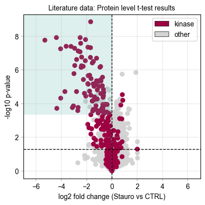
First, inspect the aggregated protein results for the standard t-test

fig, axm = at.pl.create_figure(1, 1, figsize=(4, 4))
ax = axm.next()

at.pl.Plots.scatter(
    ax=ax,
    data=tt_protein_table,
    x_column="log2fc",
    y_column="-log10(p_value)",
    xlim=(-7, 7),
    color_map_column="kinase_status",
    color_dict=color_dict,
    legend="auto",
)

at.pl.add_lines(
    ax=ax,
    intercepts=[0],
    linetype="vline",
    linestyle="--",
)

at.pl.add_lines(
    ax=ax,
    intercepts=[-np.log10(0.05)],
    linetype="hline",
    linestyle="--",
)

at.pl.label_axes(
    ax=ax,
    xlabel="log2 fold change (Stauro vs CTRL)",
    ylabel="-log10 p-value",
    title="Literature data: Protein level t-test results",
)

# We draw a rectangle to indicate the kinase scoring threshold

ttest_ks_result = kinase_score(tt_protein_table, id_col="genes", threshold=0.8)
if ttest_ks_result:
    rect = Rectangle(
        xy=(-7, ttest_ks_result["threshold"]),  # Bottom-left corner
        width=7,  # Width to cover from -7 to 0 (downregulated region)
        height=tt_protein_table["-log10(p_value)"].max()
        + 0.5
        - ttest_ks_result["threshold"],  # Height with small padding
        linewidth=2,
        facecolor=at.pl.BaseColors.get("green", alpha=0.2),
    )
    print(
        f"Kinase scoring threshold at -log10(p_value) = {ttest_ks_result['threshold']:.2f}, covering {ttest_ks_result['n_candidates']} proteins with {ttest_ks_result['n_kinases']} kinases ({ttest_ks_result['kinase_percentage'] * 100:.1f}%)"
    )
    ax.add_patch(rect)

# save figure
at.pl.save_figure(
    fig=fig,  # Note that here we're using the whole figure to whose axes we added our plots
    filename="Literature_PELSA_TTEST_AggProt_Stauro.svg",
    output_dir="./example_outputs",
)

Total unique kinases in the dataset: 276
Total unique kinases in the downregulated dataset: 215
Kinase scoring threshold at -log10(p_value) = 3.34, covering 108.0 proteins with 87.0 kinases (80.6%)

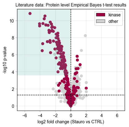
Next, inspect the protein-aggregated results from the Empirical Bayes moderated ttest (Limma-like)

fig, axm = at.pl.create_figure(1, 1, figsize=(4, 4))
ax = axm.next()

at.pl.Plots.scatter(
    ax=ax,
    data=eb_protein_table,
    x_column="log2fc",
    y_column="-log10(p_value)",
    xlim=(-7, 7),
    color_map_column="kinase_status",
    color_dict=color_dict,
    legend="auto",
)

at.pl.add_lines(
    ax=ax,
    intercepts=[0],
    linetype="vline",
    linestyle="--",
)

at.pl.add_lines(
    ax=ax,
    intercepts=[-np.log10(0.05)],
    linetype="hline",
    linestyle="--",
)

at.pl.label_axes(
    ax=ax,
    xlabel="log2 fold change (Stauro vs CTRL)",
    ylabel="-log10 p-value",
    title="Literature data: Protein level Empirical Bayes t-test results",
)

# We draw a rectangle to indicate the kinase scoring threshold

ebayes_ttest_ks_results = kinase_score(eb_protein_table, id_col="genes", threshold=0.8)
if ebayes_ttest_ks_results:
    rect = Rectangle(
        xy=(-7, ebayes_ttest_ks_results["threshold"]),  # Bottom-left corner
        width=7,  # Width to cover from -7 to 0 (downregulated region)
        height=eb_protein_table["-log10(p_value)"].max()
        + 0.5
        - ebayes_ttest_ks_results["threshold"],  # Height with small padding
        linewidth=2,
        facecolor=at.pl.BaseColors.get("green", alpha=0.2),
    )
    print(
        f"Kinase scoring threshold at -log10(p_value) = {ebayes_ttest_ks_results['threshold']:.2f}, covering {ebayes_ttest_ks_results['n_candidates']} proteins with {ebayes_ttest_ks_results['n_kinases']} kinases ({ebayes_ttest_ks_results['kinase_percentage'] * 100:.1f}%)"
    )
    ax.add_patch(rect)

# save figure
at.pl.save_figure(
    fig=fig,  # Note that here we're using the whole figure to whose axes we added our plots
    filename="Literature_PELSA_EBAYES_TTEST_AggProt_Stauro.svg",
    output_dir="./example_outputs",
)

Total unique kinases in the dataset: 253
Total unique kinases in the downregulated dataset: 197
Kinase scoring threshold at -log10(p_value) = 3.57, covering 117.0 proteins with 94.0 kinases (80.3%)

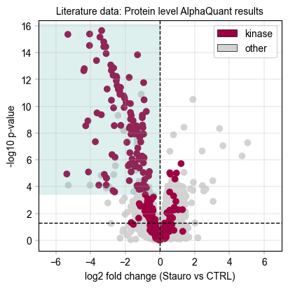
Next, inspect the protein-aggregated results from Alphaquant

import numpy as np

fig, axm = at.pl.create_figure(1, 1, figsize=(4, 4))
ax = axm.next()

at.pl.Plots.scatter(
    ax=ax,
    data=aq_protein_table,
    x_column="log2fc",
    y_column="-log10(p_value)",
    xlim=(-7, 7),
    color_map_column="kinase_status",
    color_dict=color_dict,
    legend="auto",
)

at.pl.add_lines(
    ax=ax,
    intercepts=[0],
    linetype="vline",
    linestyle="--",
)

at.pl.add_lines(
    ax=ax,
    intercepts=[-np.log10(0.05)],
    linetype="hline",
    linestyle="--",
)

at.pl.label_axes(
    ax=ax,
    xlabel="log2 fold change (Stauro vs CTRL)",
    ylabel="-log10 p-value",
    title="Literature data: Protein level AlphaQuant results",
)

# We draw a rectangle to indicate the kinase scoring threshold
aq_ks_result = kinase_score(aq_protein_table, id_col="protein", threshold=0.8)
if aq_ks_result:
    rect = Rectangle(
        xy=(-7, aq_ks_result["threshold"]),  # Bottom-left corner
        width=7,  # Width to cover from -7 to 0 (downregulated region)
        height=aq_protein_table["-log10(p_value)"].max() + 0.5 - aq_ks_result["threshold"],  # Height with small padding
        linewidth=2,
        facecolor=at.pl.BaseColors.get("green", alpha=0.2),
    )
    print(
        f"Kinase scoring threshold at -log10(p_value) = {aq_ks_result['threshold']:.2f}, covering {aq_ks_result['n_candidates']} proteins with {aq_ks_result['n_kinases']} kinases ({aq_ks_result['kinase_percentage'] * 100:.1f}%)"
    )
    ax.add_patch(rect)

# save figure
at.pl.save_figure(
    fig=fig,  # Note that here we're using the whole figure to whose axes we added our plots
    filename="Literature_PELSA_AlphaQuant_AggProt_Stauro.svg",
    output_dir="./example_outputs",
)

Total unique kinases in the dataset: 276
Total unique kinases in the downregulated dataset: 215
Kinase scoring threshold at -log10(p_value) = 3.40, covering 137.0 proteins with 110.0 kinases (80.3%)

Visualize the kinase enrichment results compared to literature data

In Figure 2 b of Kejia, Li et al., the number of downregulated vs. kinase proteins at 80 % specificity (as computed above) is given at 135 downregulated candidates and 108 kinase targets. Note that their result were computed using an Empirical Bayes test. We can visualize this data and compare to our alphapepttools differential expression data:

total_candidates = pd.DataFrame(
    {
        "group": ["EB [Lit]", "alphapepttools t-test", "alphapepttools EBayes t-test", "alphapepttools\nAlphaQuant"],
        "value": [
            135,
            ttest_ks_result["n_candidates"],
            ebayes_ttest_ks_results["n_candidates"],
            aq_ks_result["n_candidates"],
        ],
    }
)

total_kinases = pd.DataFrame(
    {
        "group": ["EB [Lit]", "alphapepttools t-test", "alphapepttools EBayes t-test", "alphapepttools\nAlphaQuant"],
        "value": [108, ttest_ks_result["n_kinases"], ebayes_ttest_ks_results["n_kinases"], aq_ks_result["n_kinases"]],
    }
)

color_dict = {
    "candidates": at.pl.BaseColors.get("green"),
    "kinases": at.pl.BaseColors.get("red", lighten=0.1, alpha=0.8),
}

fig, axm = at.pl.create_figure(1, 1, figsize=(6, 4))

# First, plot the total candidates
ax = axm.next()
ax.set_ylim(0, 175)

at.pl.Plots.barplot(
    ax=ax,
    data=total_candidates,
    grouping_column="group",
    value_column="value",
    color=at.pl.BaseColors.get("green"),
)

at.pl.label_plot(
    ax=ax,
    x_values=range(1, len(total_candidates) + 1),
    y_values=total_candidates["value"].tolist(),
    labels=total_candidates["value"].astype(str).tolist(),
    label_kwargs={"va": "bottom", "ha": "center"},
)

# Then, add the kinases
at.pl.Plots.barplot(
    ax=ax,
    data=total_kinases,
    grouping_column="group",
    value_column="value",
    color=at.pl.BaseColors.get("red", lighten=0.3),
)

at.pl.label_plot(
    ax=ax,
    x_values=range(1, len(total_kinases) + 1),
    y_values=total_kinases["value"].tolist(),
    labels=total_kinases["value"].astype(str).tolist(),
    label_kwargs={"va": "bottom", "ha": "center"},
)

at.pl.label_axes(
    ax=ax,
    xlabel="",
    ylabel="Number of candidates",
    title="Kinase enrichment candidates",
)

at.pl.add_legend_to_axes(
    ax=ax,
    levels=color_dict,
)

# save figure
at.pl.save_figure(
    fig=fig,  # Note that here we're using the whole figure to whose axes we added our plots
    filename="Literature_PELSA_Kinase_Enrichment_Candidates_Comparison.svg",
    output_dir="./example_outputs",
)

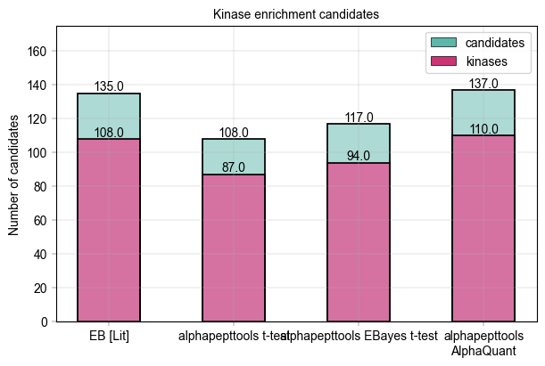
In summary, we saw that alphapepttools…

• can swiftly load precursor and protein data into AnnData instances

• contains standardized, ‘plug and play’ modules for proteomics differential expression

• Equals/outperforms the empirical Bayes approach from literature, demonstrating that we have a strong framework for analysing PELSA-data in-house using AlphaQuant.