Watch evidence become a study matrix#
FastaLake makes three different decisions: which complete protein sequences to search, how to report accepted peptide evidence, and how to combine its measured intensities. Follow them below with small, invented examples.
Use Next to inspect a step, or Play to run the explanation. Nothing plays automatically. Written steps and downloadable stills give the same explanation without animation. Letters are illustrative protein accessions; peptide labels stand for distinct sequences, not spectra or intensities.
| Decision | Input | Output | Rule |
|---|---|---|---|
| Selection parsimony, before search | Predicted peptides mapped onto candidate proteins | A compact target FASTA | Fixed unique and total evidence counts; deterministic hash ties |
| Study grouping, after search | Accepted target peptides and their reported proteins across a declared study | A peptide-to-group dictionary | Repeatedly explain the most uncovered peptides; lexical ties |
| Sum aggregation | Positive finite LFQ features passing the local peptide acceptance gate | A group-by-acquisition matrix | Assign through the dictionary; sum each included feature once |
1. Which candidates survive selection parsimony?#
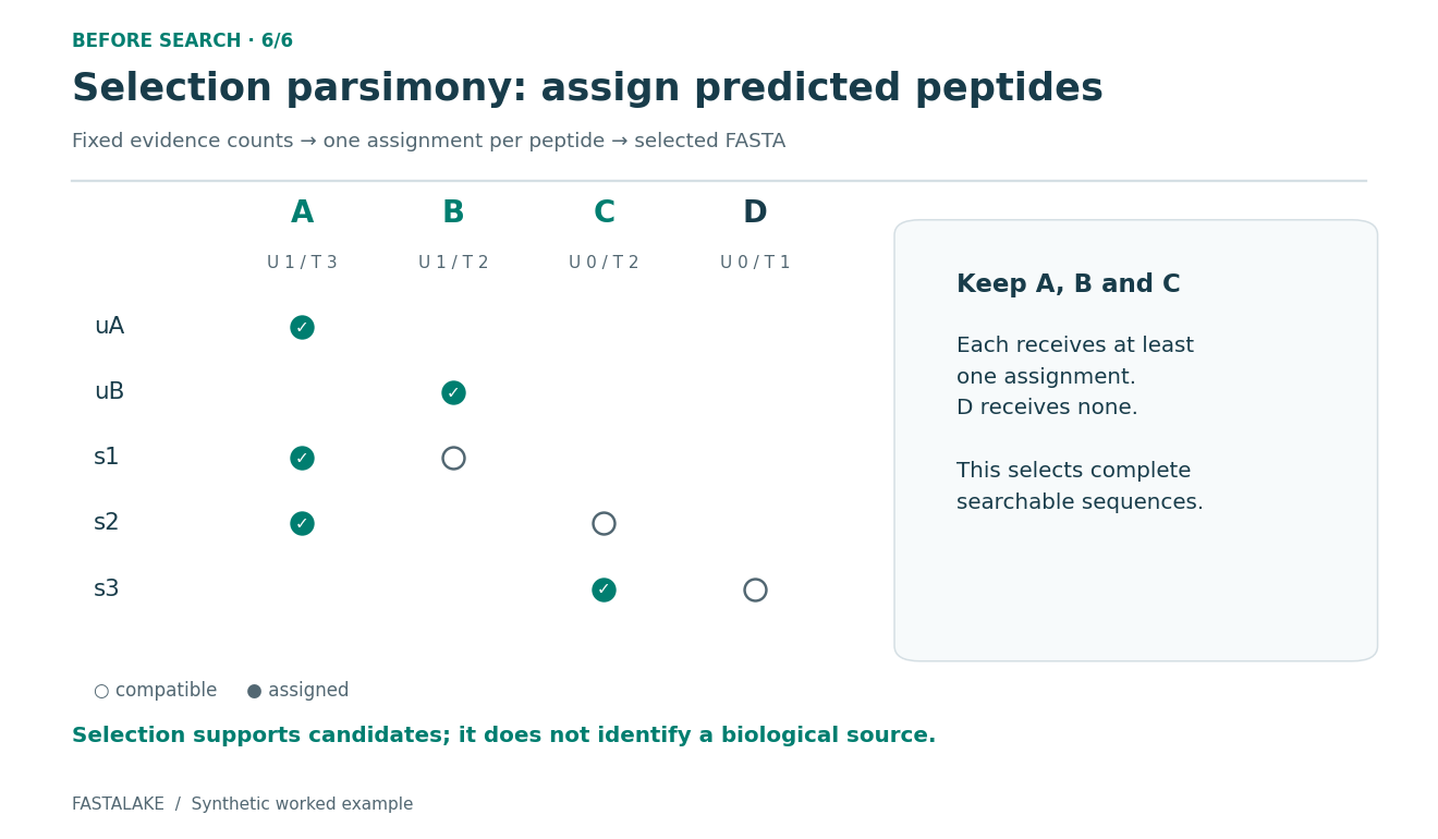
A protein does not need a unique peptide to survive. It needs to receive an assignment. The example deliberately includes C, supported only by shared peptides.
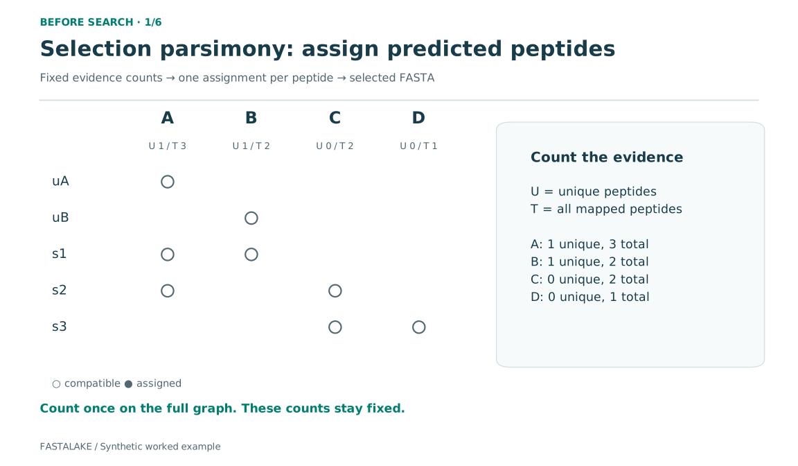
- Count each protein's unique mapped peptides (U) and total distinct mapped peptides (T) on the whole graph. These counts stay fixed.
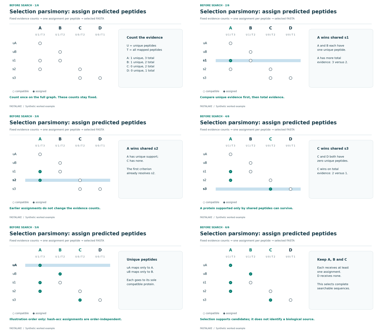
- Assign shared s1 to A: A and B tie on U, but A has more total evidence.
- Assign s2 to A: A has unique support; C has none.
- Assign s3 to C: C and D have no unique support, but C has more total evidence.
- Assign uA to A and uB to B, their sole compatible proteins.
- Retain complete proteins A, B and C. D receives no assignment.
If U and T both tie, the supported runner uses the smallest 64-bit FNV-1a hash
of the accession, followed by lexical order for a remaining hash collision.
This tie rule is distinct from the SHA-256 identity of a protein sequence.
Presentation order does not affect this fixed-count hash-acc result.
Download GIF · Final still · Exact rule and identity conventions
2. How does study parsimony build a common dictionary?#
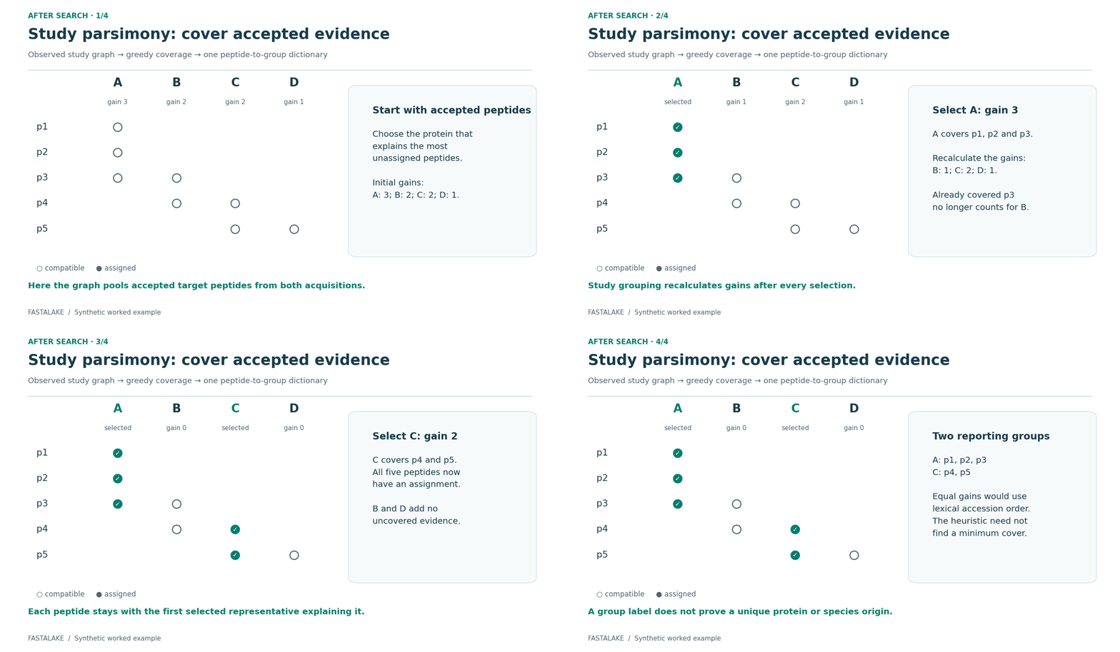
Now use a different graph, built from accepted search peptides. The study rule keeps track of evidence already covered; its gains change after selection.
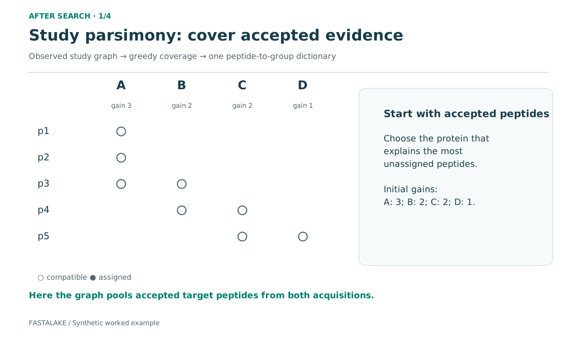
- A explains three uncovered peptides; B and C each explain two; D explains one.
- Select A and assign p1, p2 and p3. B now adds only p4, while C adds p4 and p5.
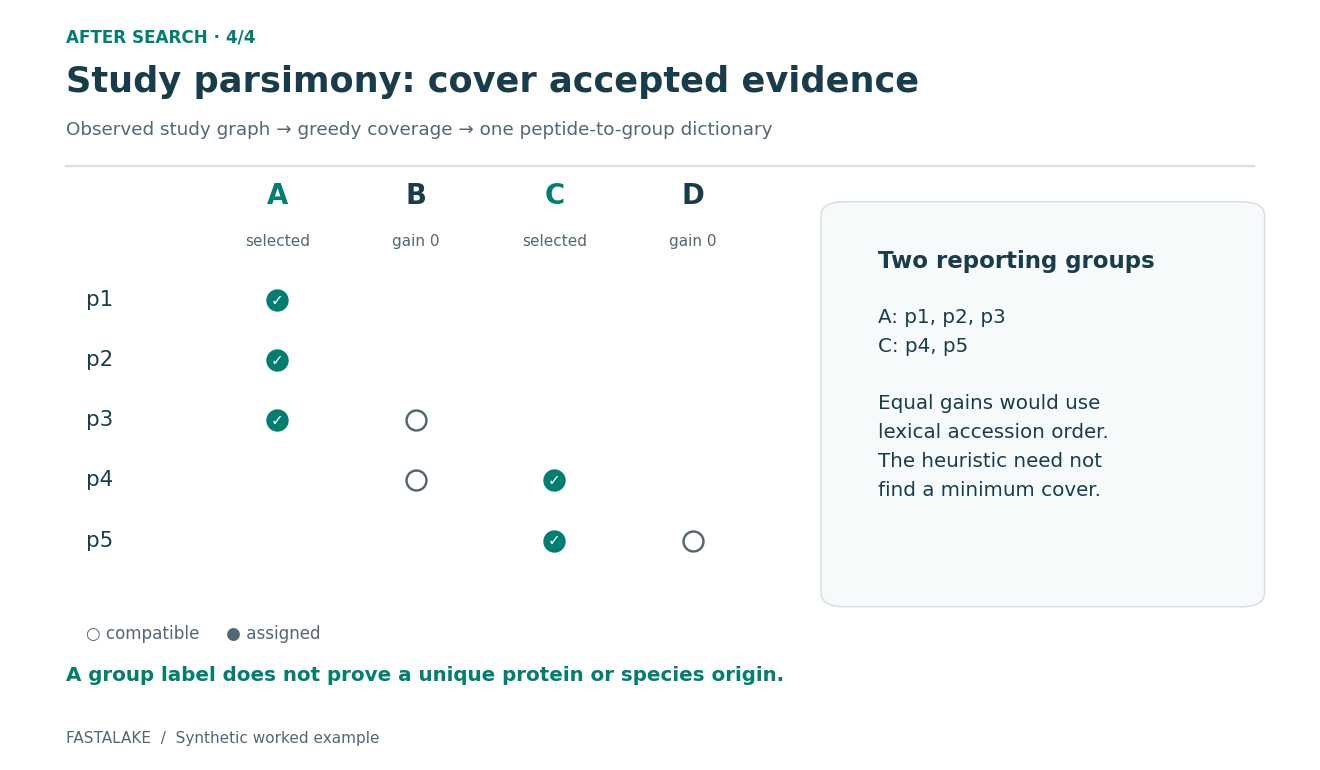
- Select C and assign p4 and p5. Every observed peptide is covered.
- Report groups A and C. Equal gains use lexical accession order. This greedy procedure need not produce the smallest possible cover.
The first selected representative explaining a peptide keeps its assignment. The declared study roster matters: changing the accepted graph can change the dictionary. Preserve full local memberships as well as the group label.
Download GIF · Final still · Output contract
3. How do measured features become quantities?#
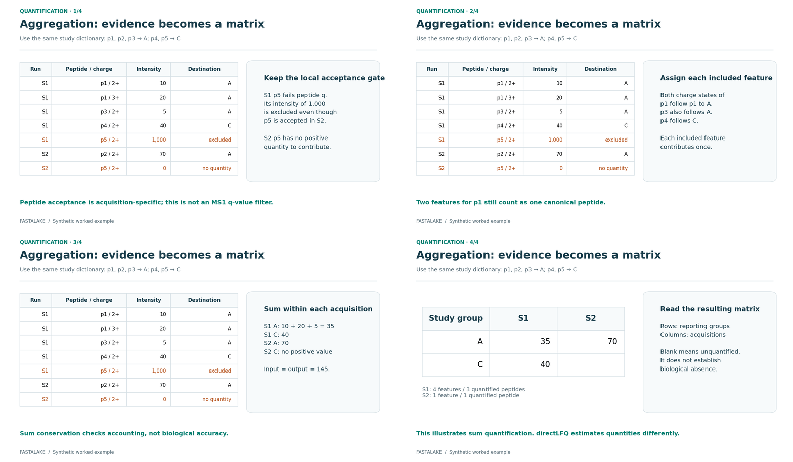
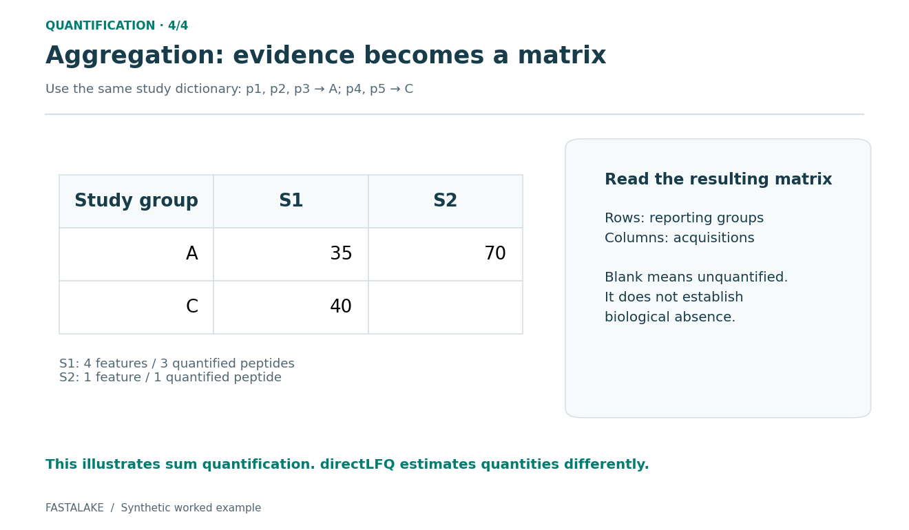
Use that same dictionary: p1–p3 belong to A, p4–p5 to C. Each included LFQ feature contributes once, within its own acquisition. Multiple charges or modifications can contribute to one canonical peptide.
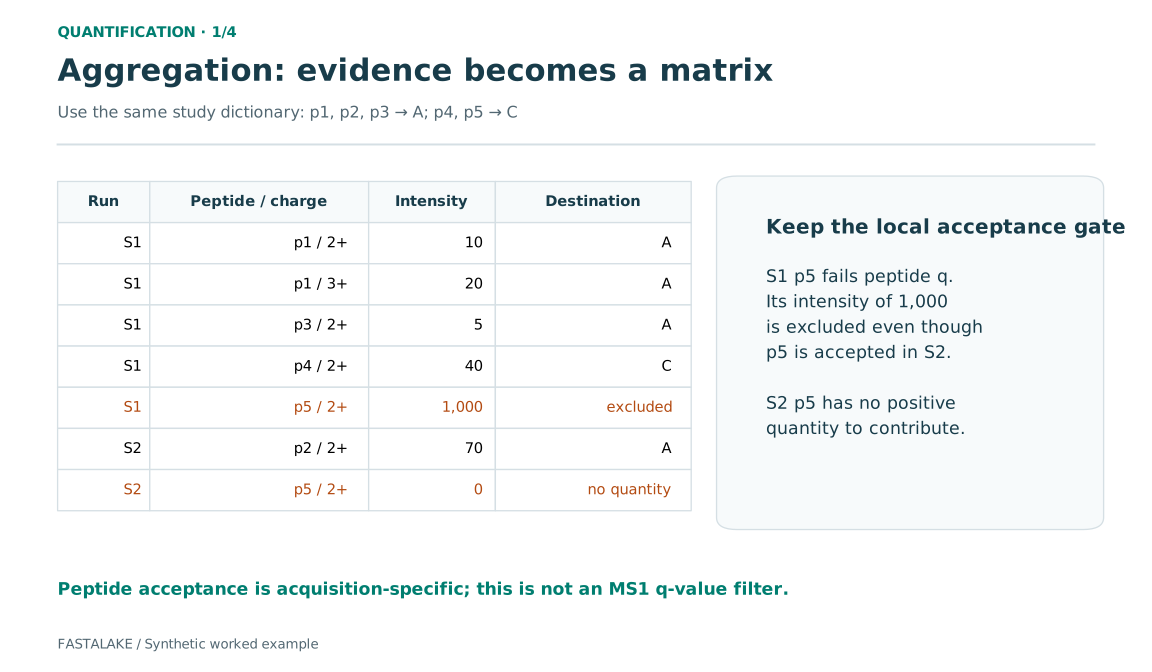
- S1 accepts p1, p3 and p4 at target peptide q ≤ 0.01. S1 p5 has q = 0.20; its intensity of 1,000 is excluded. Acceptance of p5 in S2 cannot rescue it.
- In S1, p1 contributes two features (10 and 20), and p3 contributes 5 to A. p4 contributes 40 to C. In S2, p2 contributes 70 to A; accepted p5 has zero intensity, so it supplies identification evidence but no positive quantity.
- The matrix is A = (35, 70), C = (40, blank). Included input and output intensity both total 145. A blank cell means unquantified, not biological absence.
This is the study utility's default sum route. Its acceptance gate is the
search's target peptide q value, not an additional cutoff on the MS1 LFQ
q_value. directLFQ uses the same assignments
but estimates quantities differently; it is not described by this sum example.
Download GIF · Final still · Read the actual output files
Try it and inspect the evidence#
Run the two-acquisition CAMPI example, then open
the selected FASTA, peptide_to_study_group.tsv, feature_assignments.tsv.gz
and study_group_matrix.tsv. Those files let you follow a peptide through the
same decisions on measured data.
To regenerate these illustrations from the repository root:
Use a new output directory and the documentation Python environment. The script
executes study_dictionary and group_searches on synthetic inputs, checks the
displayed matrix and conserved intensity, and records source hashes in
CHECK.json. The razor animation is a teaching trace of the Rust comparator;
rendering it does not execute the native engine or validate scientific accuracy.