A walk through the scPortrait Ecosystem
This notebook will introduce you to the scPortrait ecosystem and give you a complete working example of how to use scPortrait. It will walk you through the following steps of the scPortrait workflow: 1. segmentation: Generates masks for the segmentation of input images into individual cells 2. extraction: The segmentation masks are applied to extract single-cell images for all cells in the input images. Images of individual cells are rescaled to [0, 1] per channel. 3. classification:
The image-based phenotype of each individual cell in the extracted single-cell dataset is classified using the specified classification method. Multiple classification runs can be performed on the same dataset using different classification methods. Here we utilize the pretrained binary classifier from the original SPARCS manuscript that identifies individual cells defective in a biological process called “autophagy”. 4. selection: Cutting
instructions for the isolation of selected individual cells by laser microdissection are generated. The cutting shapes are written to an .xml file which can be loaded on a leica LMD microscope for automated cell excision.
The data used in this notebook was previously stitched using the stitching workflow in SPARCStools. Please see the notebook here.
Import Required Libraries
First we need to import all of the python functions we require to run the pipeline.
[1]:
import os
import numpy as np
import matplotlib.pyplot as plt
from tqdm.notebook import tqdm
import pandas as pd
import h5py

from scportrait.pipeline.project import Project
from scportrait.pipeline.segmentation.workflows import WGASegmentation
from scportrait.pipeline.extraction import HDF5CellExtraction
from scportrait.pipeline.classification import MLClusterClassifier
from scportrait.pipeline.selection import LMDSelection
/Users/sophia/mambaforge/envs/scPortrait/lib/python3.10/site-packages/tqdm/auto.py:21: TqdmWarning: IProgress not found. Please update jupyter and ipywidgets. See https://ipywidgets.readthedocs.io/en/stable/user_install.html
  from .autonotebook import tqdm as notebook_tqdm
Generate the Project Structure
Executing this code will generate a new scPortrait project in the designated location. Each scPortrait project has the following general structure:
.
├── classification
│   └── classifier_name
│       └── processing.log
├── config.yml
├── extraction
├── segmentation
└── processing.log
[2]:
project_location = f"../../../example_data/example_1/project"

project = Project(os.path.abspath(project_location),
                  config_path= "../../../example_data/example_1/config_example1.yml",
                  overwrite=True,
                  debug=True,
                  segmentation_f=WGASegmentation,
                  extraction_f=HDF5CellExtraction,
                  classification_f=MLClusterClassifier,
                  selection_f=LMDSelection
                  )
Updating project config file.
[11/09/2024 17:10:07] Loading config from /Users/sophia/Documents/GitHub/scPortrait/example_data/example_1/project/config.yml
/Users/sophia/Documents/GitHub/scPortrait/src/scportrait/pipeline/project.py:107: UserWarning: There is already a directory in the location path
  warnings.warn("There is already a directory in the location path")
[11/09/2024 17:10:07] No cache directory specified in config using current working directory /Users/sophia/Documents/GitHub/scPortrait/docs_source/pages/notebooks.
Load Imaging Data
Once we have generated our project structure we next need to load our imaging data. There are several different ways to do this.
you can load the images directly from file by specifying a list of filepaths
you can load the images from numpy arrays that are already loaded into memory
Here it is important that you load the channels in the following order: Nucleus, Cellmembrane, others
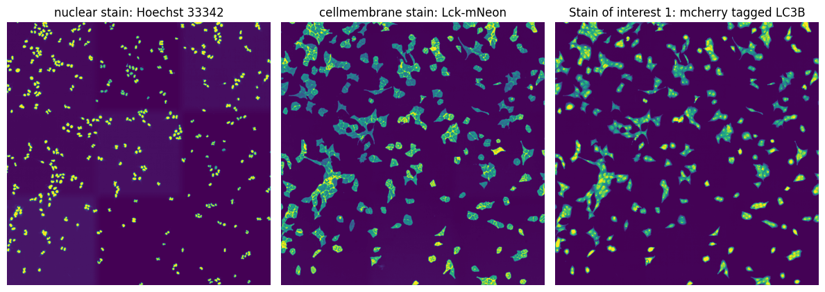
In this particular example we are utilizing images from U2OS cells which are stained with Hoechst 33342 to visualize nuclei and express Lck-mNeon to visualize the cellular membrane and LC3B-mcherry, a fluroescently tagged protein relevant for visualizing the biological process of autophagy. The cells have not been stimulated to induce autophagy and should be autophagy defective.
Method 1: loading images from file
[3]:
images = ["../../../example_data/example_1/input_images/Ch1.tif",
          "../../../example_data/example_1/input_images/Ch2.tif",
          "../../../example_data/example_1/input_images/Ch3.tif"]

project.load_input_from_tif_files(images)
[11/09/2024 17:10:07] Output location /Users/sophia/Documents/GitHub/scPortrait/example_data/example_1/project/sparcs.sdata already exists. Overwriting.
INFO     The Zarr backing store has been changed from None the new file path:
         /Users/sophia/Documents/GitHub/scPortrait/example_data/example_1/project/sparcs.sdata
[11/09/2024 17:10:08] Initialized temporary directory at /Users/sophia/Documents/GitHub/scPortrait/docs_source/pages/notebooks/Project_ytcnwjya for Project
[11/09/2024 17:10:08] Image input_image written to sdata object.
[11/09/2024 17:10:08] Cleaned up temporary directory at <TemporaryDirectory '/Users/sophia/Documents/GitHub/scPortrait/docs_source/pages/notebooks/Project_ytcnwjya'>
Method 2: loading images from numpy array
To simulate the case where the images you want to load are already loaded as a numpy array, we first convert the images to a numpy array and then pass this array to the project instead of only providing the image paths.
[4]:
from tifffile import imread

images = ["../../../example_data/example_1/input_images/Ch1.tif",
          "../../../example_data/example_1/input_images/Ch2.tif",
          "../../../example_data/example_1/input_images/Ch3.tif"]

image_arrays = np.array([imread(path) for path in images])

project.load_input_from_array(image_arrays)
[11/09/2024 17:10:08] Output location /Users/sophia/Documents/GitHub/scPortrait/example_data/example_1/project/sparcs.sdata already exists. Overwriting.
INFO     The Zarr backing store has been changed from None the new file path:
         /Users/sophia/Documents/GitHub/scPortrait/example_data/example_1/project/sparcs.sdata
[11/09/2024 17:10:08] Image input_image written to sdata object.
Looking at the loaded images
The loaded images are accesible via the input_image parameter of the project. They are saved into the underlying spatialdata object.
[5]:
project.input_image
[5]:
<xarray.DataArray 'image' (c: 3, y: 3040, x: 3038)> Size: 55MB
dask.array<from-zarr, shape=(3, 3040, 3038), dtype=uint16, chunksize=(1, 1000, 1000), chunktype=numpy.ndarray>
Coordinates:
  * c        (c) <U9 108B 'channel_0' 'channel_1' 'channel_2'
  * y        (y) float64 24kB 0.5 1.5 2.5 3.5 ... 3.038e+03 3.038e+03 3.04e+03
  * x        (x) float64 24kB 0.5 1.5 2.5 3.5 ... 3.036e+03 3.036e+03 3.038e+03
Attributes:
transform: {'global': Identity }[6]:
# visualize input images as example
# it is not recommended to execute this block with large input images as it will compute for some time

fig, axs = plt.subplots(1, 3, figsize = (12, 6));
axs[0].imshow(project.input_image[0]);
axs[0].axis("off");
axs[0].set_title("nuclear stain: Hoechst 33342")

axs[1].imshow(project.input_image[1]);
axs[1].axis("off");
axs[1].set_title("cellmembrane stain: Lck-mNeon")

axs[2].imshow(project.input_image[2]);
axs[2].axis("off");
axs[2].set_title("Stain of interest 1: mcherry tagged LC3B")

fig.tight_layout()
[7]:
#alternatively you can also visualize the input images as well as all other objects saved in spatialdata object

project.view_sdata()
Generating a Segmentation
scPortrait has different segmentation workflows between which you can choose. If none of them fit your needs you can also easily write your own.
Here we will demonstrate the CPU based classical segmentation method that was also utilized in the manuscript.
We define the segmentation method to be used when we initialize the project. In this case we used the WGASegmentation method. The ShardedWGASegmentation works very similarily but allows you to process several image chunks in parallel for more efficient computation on large input images.
By specifying debug = True we can see intermediate output results from the segmentation.
The WGASegmentation method relies on parameters specified in the config.yml we loaded when initializing our project.
WGASegmentation:
input_channels: 3
cache: "."
chunk_size: 50 # chunk size for chunked HDF5 storage
lower_quantile_normalization:   0.001
upper_quantile_normalization:   0.999
median_filter_size:   4 # Size in pixels
nucleus_segmentation:
    lower_quantile_normalization:   0.01 # quantile normalization of dapi channel before local tresholding Strong normalization (0.05,0.95) can help with nuclear speckles.
    upper_quantile_normalization:   0.99 # quantile normalization of dapi channel before local tresholding.Strong normalization (0.05,0.95) can help with nuclear speckles.
    median_block: 41 # Size of pixel disk used for median, should be uneven
    median_step: 4
    threshold: 0.2 # threshold above local median for nuclear segmentation
    min_distance: 8 # minimum distance between two nucleis in pixel
    peak_footprint: 7 #
    speckle_kernel: 9 # Erosion followed by Dilation to remove speckels, size in pixels, should be uneven
    dilation: 0 # final dilation of pixel mask
    min_size: 200 # minimum nucleus area in pixel
    max_size: 1000 # maximum nucleus area in pixel
    contact_filter: 0.5 # minimum nucleus contact with background
cytosol_segmentation:
    threshold: 0.05 # treshold above which cytosol is detected
    lower_quantile_normalization: 0.01
    upper_quantile_normalization: 0.99
    erosion: 2 # erosion and dilation are used for speckle removal and shrinking / dilation
    dilation: 7 # for no change in size choose erosion = dilation, for larger cells increase the mask erosion
    min_clip: 0
    max_clip: 0.2
    min_size: 200
    max_size: 6000
chunk_size: 50
filter_masks_size: True
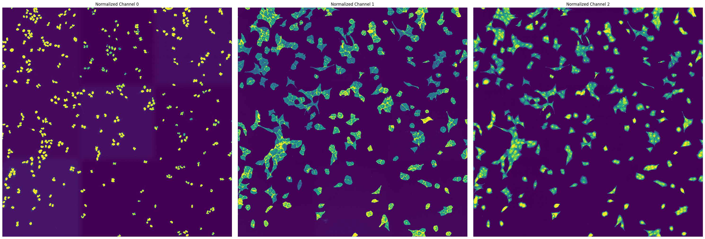
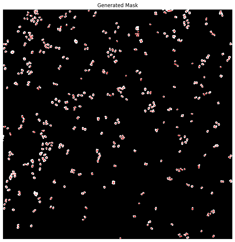
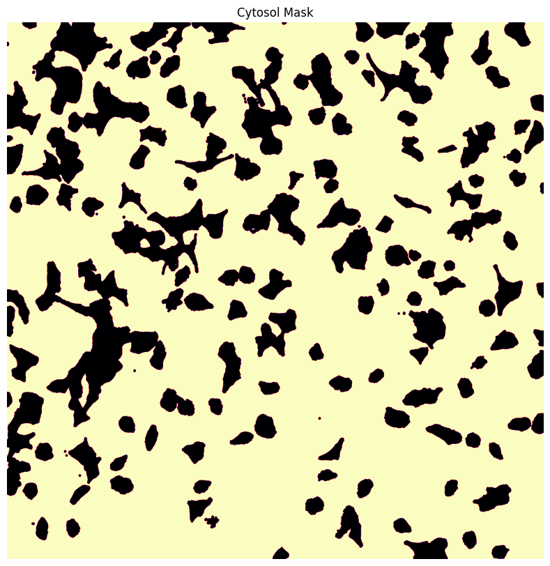
By passing the parameter debug = True we tell scPortrait to also generate intermediate outputs which we can look at to see the different segmentation steps. It is only recommended to do this for debugging or visualization purposes as it will utilize more memory and be slower.
For the WGASegmentation method the intermediate outputs that are displayed are the following:
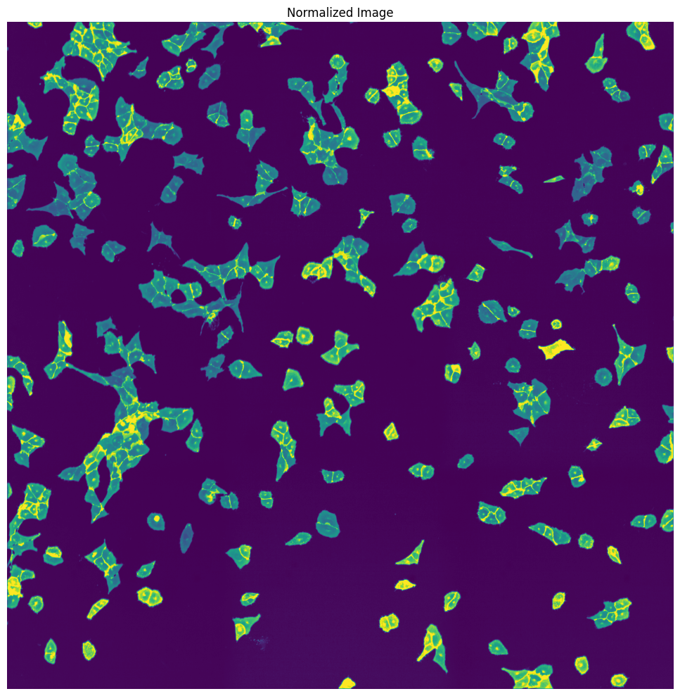
percentile normalized input images for each of the three channels (3 images)
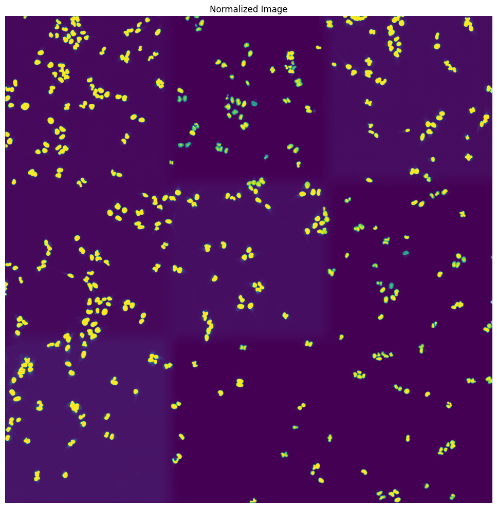
median normalized input images (this slightl smooths the images for a better segmentation result) (3 images)
histogram showing the intensity distribution for nuclear and cytosolic channel (2 plots)
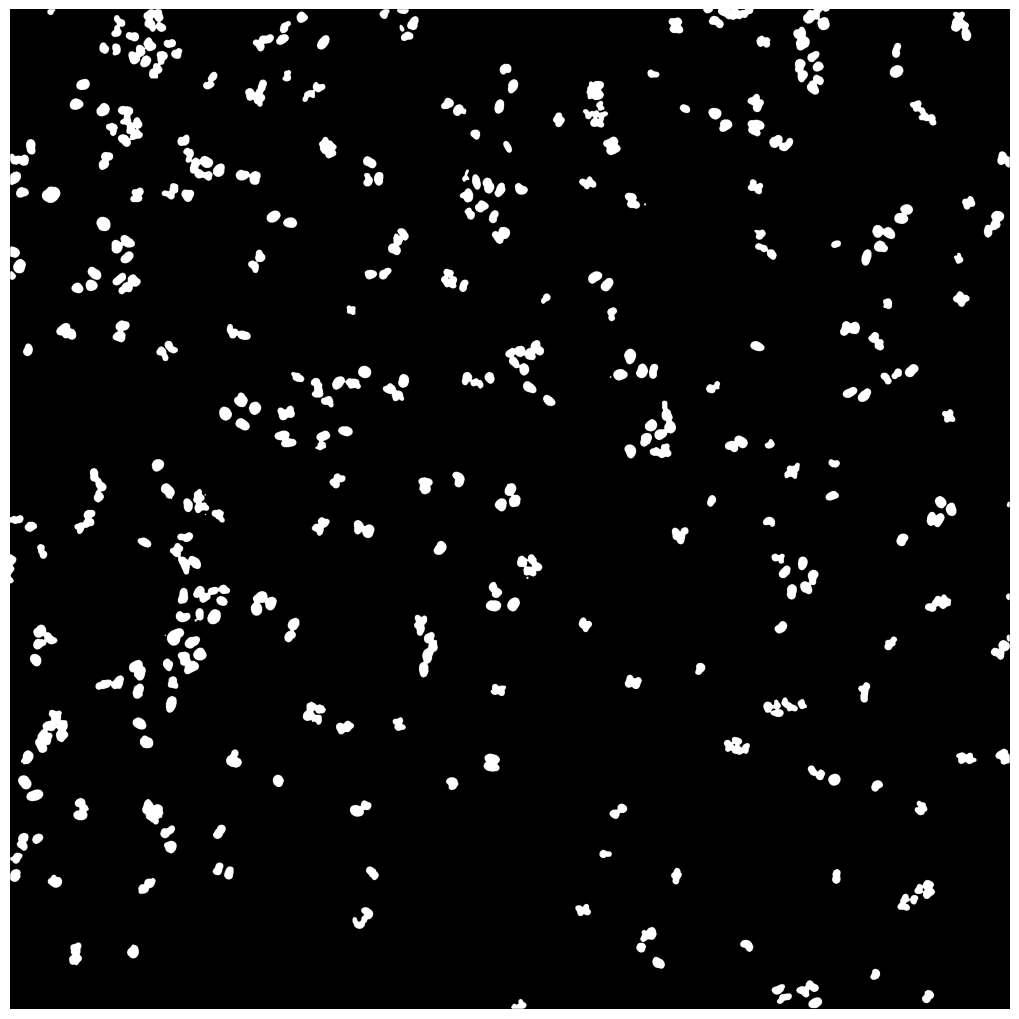
generated mask after applying nuclear thresholding
nuclear thresholding mask with calculated centers for each detected nucleus
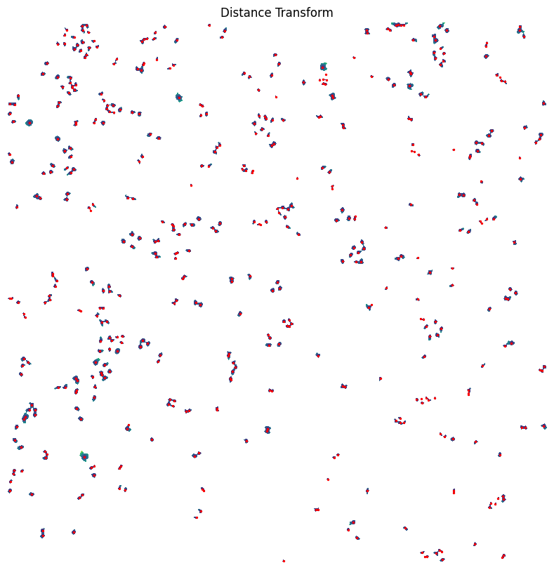
fast marching map with nuclei centers indicated in red
segmented individual nuclei (2 different visualizations)
starting nucleus mask for filtering
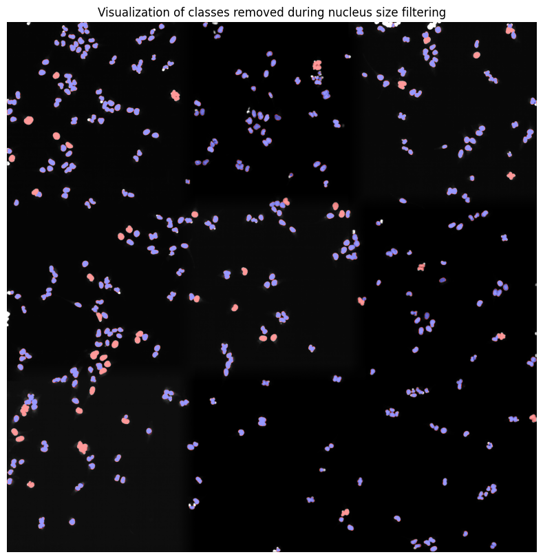
histrogram showing size distribution of segmented nuclei
segmentation mask with too small nuclei shown in red
segmentation mask with too large nuclei shown in red
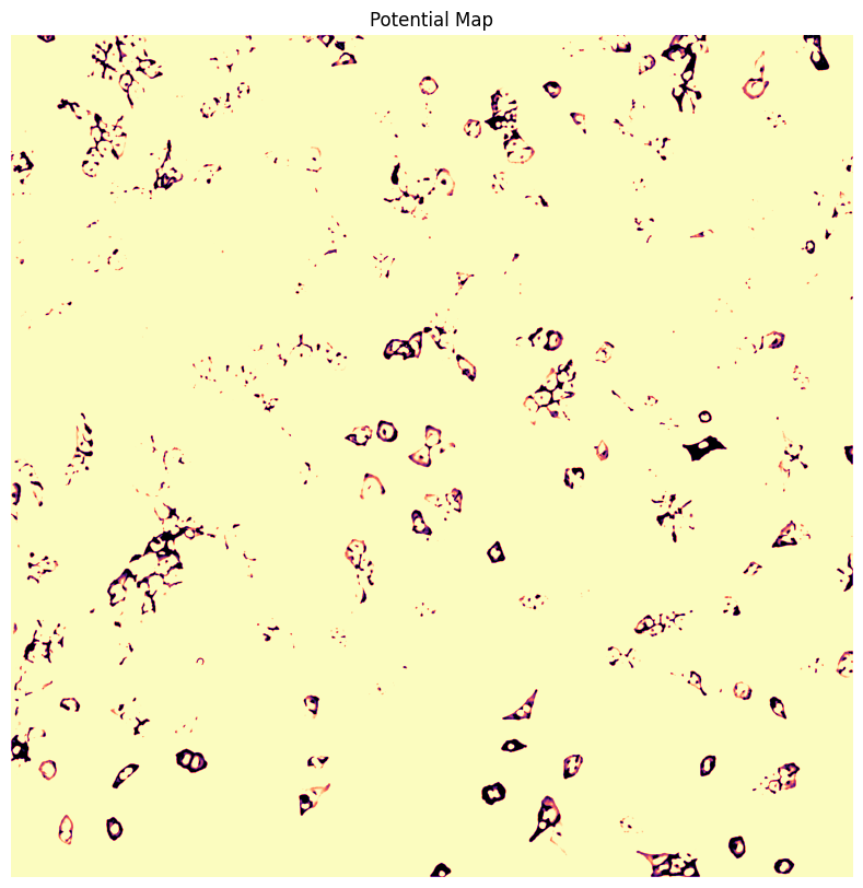
WGA thresholding mask
WGA potential map
WGA fast marching results
Watershed results with nuclear centers shown in red
WGA mask
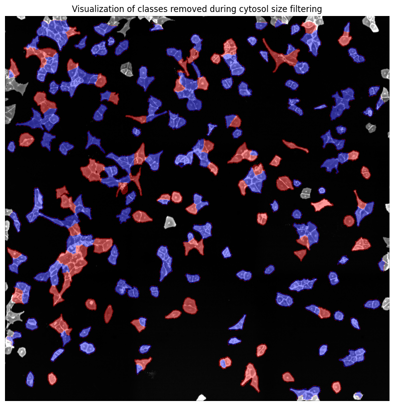
Cytosol size distribution
cytosol mask with too small cells shown in red
cytosol mask with too large cells shown in red
[8]:
project.segment()
[11/09/2024 17:10:19] Initialized temporary directory at /var/folders/35/p4c58_4n3bb0bxnzgns1t7kh0000gn/T/./WGASegmentation_959o1ov3 for WGASegmentation
[11/09/2024 17:10:19] Normalization of the input image will be performed.
[11/09/2024 17:10:19] Normalizing each channel to the same range
[11/09/2024 17:10:21] Performing median filtering on input image
[11/09/2024 17:10:35] Percentile normalization of nucleus input image to range 0.01, 0.99
[11/09/2024 17:10:35] Normalizing each channel to the same range
[11/09/2024 17:10:35] Using local thresholding with a threshold of 0.2 to calculate nucleus mask.

[11/09/2024 17:10:51] Performing filtering of nucleus with specified thresholds [200, 1000] from config file.
[11/09/2024 17:10:51] Removed 47 nuclei as they fell outside of the threshold range [200, 1000].
[11/09/2024 17:10:52] Total time to perform nucleus size filtering: 0.7049751281738281 seconds
OMP: Info #276: omp_set_nested routine deprecated, please use omp_set_max_active_levels instead.
[11/09/2024 17:10:53] Filtered out 6 nuclei due to contact filtering.
[11/09/2024 17:10:53] Normalizing each channel to the same range
[11/09/2024 17:10:56] Cytosol Potential Mask generated.
[11/09/2024 17:10:58] Performing filtering of cytosol with specified thresholds [200, 6000] from config file.
[11/09/2024 17:10:59] Removed 78 nuclei as they fell outside of the threshold range [200, 6000].
[11/09/2024 17:11:00] Total time to perform cytosol size filtering: 1.9455931186676025 seconds
Channels shape:  (2, 3040, 3038)
[11/09/2024 17:11:02] Segmentation seg_all_nucleus written to sdata object.
True False
[11/09/2024 17:11:02] Segmentation seg_all_cytosol written to sdata object.
True True
[11/09/2024 17:11:02] Cleaned up temporary directory at <TemporaryDirectory '/var/folders/35/p4c58_4n3bb0bxnzgns1t7kh0000gn/T/./WGASegmentation_959o1ov3'>
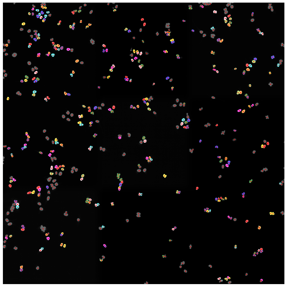
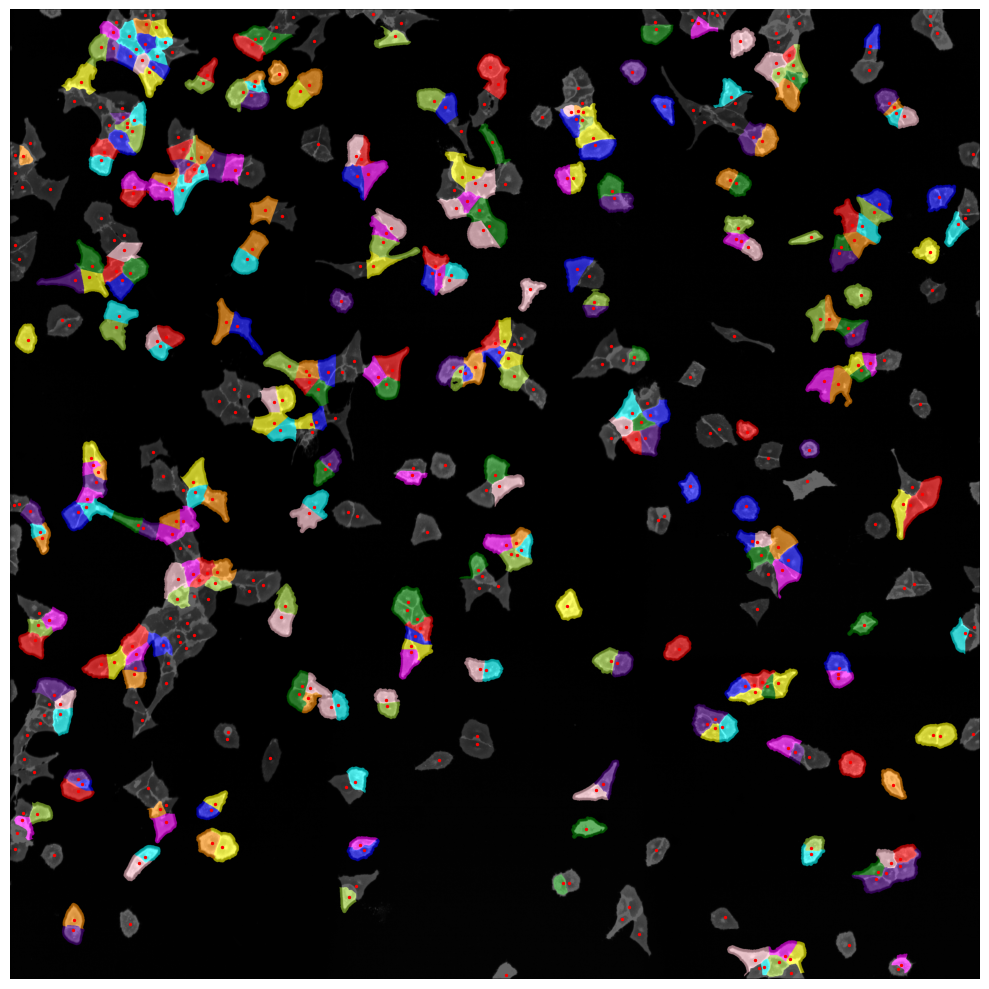
Looking at Segmentation Results
The Segmentation Results are written to a hdf5 file called segmentation.h5 located in the segmentation directory of our scPortrait project.
The file contains two datasets: channels and labels. Channels contains the input images and labels the generated segmentation masks.
[9]:
plt.figure()
plt.imshow(project.sdata.labels["seg_all_nucleus"])
plt.figure()
plt.imshow(project.sdata.labels["seg_all_cytosol"])
[9]:
<matplotlib.image.AxesImage at 0xb4b6d19c0>
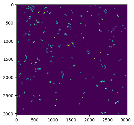
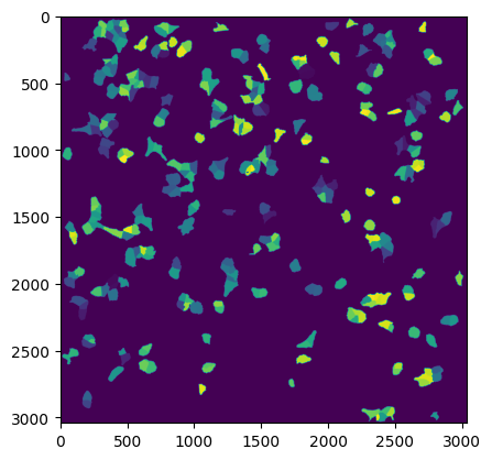
If we look at the labels dataset we can see that it contains a numpy array containing two segmentation masks: the nuclear segmentation and the cytosol segmentation generated by our chosen segmentation method.
Each segmentation mask is an array where each pixel is assigned either to background (0) or to a specific cell (cellid: whole number).
If we zoom in on the corner of the segmentation mask of a nucleus the numpy array would look like this:
[10]:
plt.imshow(project.sdata.labels["seg_all_nucleus"][230:250, 945:955])
plt.axis("off")
print(project.sdata.labels["seg_all_nucleus"][230:250, 945:955].data.compute())
[[395 395 395 395 395 395   0   0   0   0]
 [395 395 395 395 395 395 395 395   0   0]
 [395 395 395 395 395 395 395 395 395   0]
 [395 395 395 395 395 395 395 395 395   0]
 [395 395 395 395 395 395 395 395 395 395]
 [395 395 395 395 395 395 395 395 395 395]
 [395 395 395 395 395 395 395 395 395 395]
 [395 395 395 395 395 395 395 395 395 395]
 [395 395 395 395 395 395 395 395 395 395]
 [395 395 395 395 395 395 395 395 395 395]
 [395 395 395 395 395 395 395 395 395 395]
 [395 395 395 395 395 395 395 395 395   0]
 [395 395 395 395 395 395 395 395 395   0]
 [395 395 395 395 395 395 395 395   0   0]
 [395 395 395 395 395 395   0   0   0   0]
 [395 395 395 395   0   0   0   0   0   0]
 [395 395   0   0   0   0   0   0   0   0]
 [395   0   0   0   0   0   0   0   0   0]
 [  0   0   0   0   0   0   0   0   0   0]
 [  0   0   0   0   0   0   0   0   0   0]]

Extracting single-cell images
Once we have generated a segmentation mask, the next step is to extract single-cell images of segmented cells in the dataset.
Like during the segmentation there are several extraction methods to choose from. For regular scPortrait projects we need the HDF5CellExtraction method. This will extract single-cell images for all cells segmentated in the dataset and write them to a hdf5 file.
The parameters with which HDF5CellExtraction will run are again specified in the config.yml file.
HDF5CellExtraction:
    compression: True
    threads: 80 # threads used in multithreading
    image_size: 128 # image size in pixel
    cache: "."
    hdf5_rdcc_nbytes: 5242880000 # 5gb 1024 * 1024 * 5000
    hdf5_rdcc_w0: 1
    hdf5_rdcc_nslots: 50000
[11]:
project.extract()
[11/09/2024 17:11:04] Initialized temporary directory at /var/folders/35/p4c58_4n3bb0bxnzgns1t7kh0000gn/T/./HDF5CellExtraction_juskyxby for HDF5CellExtraction
[11/09/2024 17:11:04] Created new directory for extraction results: /Users/sophia/Documents/GitHub/scPortrait/example_data/example_1/project/extraction/data
[11/09/2024 17:11:04] Setup output folder at /Users/sophia/Documents/GitHub/scPortrait/example_data/example_1/project/extraction/data
[11/09/2024 17:11:04] Found 2 segmentation masks for the given key in the sdata object. Will be extracting single-cell images based on these masks: ['seg_all_nucleus', 'seg_all_cytosol']
[11/09/2024 17:11:04] Using seg_all_nucleus as the main segmentation mask to determine cell centers.
[11/09/2024 17:11:05] Points centers_cells written to sdata object.
[11/09/2024 17:11:05] Extraction Details:
[11/09/2024 17:11:05] --------------------------------
[11/09/2024 17:11:05] Number of input image channels: 3
[11/09/2024 17:11:05] Number of segmentation masks used during extraction: 2
[11/09/2024 17:11:05] Number of generated output images per cell: 5
[11/09/2024 17:11:05] Number of unique cells to extract: 328
[11/09/2024 17:11:05] Extracted Image Dimensions: 128 x 128
[11/09/2024 17:11:05] Starting single-cell image extraction of 328 cells...
[11/09/2024 17:11:05] Loading input images to memory mapped arrays...
[11/09/2024 17:11:05] Finished transferring data to memory mapped arrays. Time taken: 0.48 seconds.
[11/09/2024 17:11:05] Using batch size of 100 for multiprocessing.
[11/09/2024 17:11:05] Reducing number of threads to 4 to match number of cell batches to process.
[11/09/2024 17:11:05] Running in multiprocessing mode with 4 threads.
Processing cell batches: 100%|██████████| 4/4 [00:07<00:00,  1.77s/it]
/Users/sophia/Documents/GitHub/scPortrait/src/scportrait/pipeline/extraction.py:673: UserWarning: FigureCanvasAgg is non-interactive, and thus cannot be shown
  fig.show()
multiprocessing done.
[11/09/2024 17:11:13] Finished extraction in 7.42 seconds (44.22 cells / second)
[11/09/2024 17:11:13] Transferring results to final HDF5 data container.
[11/09/2024 17:11:13] number of cells too close to image edges to extract: 14
[11/09/2024 17:11:13] A total of 14 cells were too close to the image border to be extracted. Their cell_ids were saved to file /Users/sophia/Documents/GitHub/scPortrait/example_data/example_1/project/segmentation/removed_classes.csv.
[11/09/2024 17:11:13] Transferring extracted single cells to .hdf5
[11/09/2024 17:11:13] single-cell index created.
[11/09/2024 17:11:13] single-cell data created
[11/09/2024 17:11:13] single-cell index labelled created.
[11/09/2024 17:11:13] channel information created.
[11/09/2024 17:11:14] Benchmarking times saved to file.
[11/09/2024 17:11:14] Cleaned up temporary directory at <TemporaryDirectory '/var/folders/35/p4c58_4n3bb0bxnzgns1t7kh0000gn/T/./HDF5CellExtraction_juskyxby'>
Look at extracted single-cell images
The extracted single-cell images are written to a h5py file single_cells.h5 located under extraction\data within the project folder.
The file contains two datasets: single_cell_data and single_cell_index. single_cell_data contains the extracted single cell images while single_cell_index contains the cell id of the extracted cell at that location.
[12]:
with h5py.File(f"{project_location}/extraction/data/single_cells.h5") as hf:
    print(hf.keys())
<KeysViewHDF5 ['channel_information', 'single_cell_data', 'single_cell_index', 'single_cell_index_labelled']>
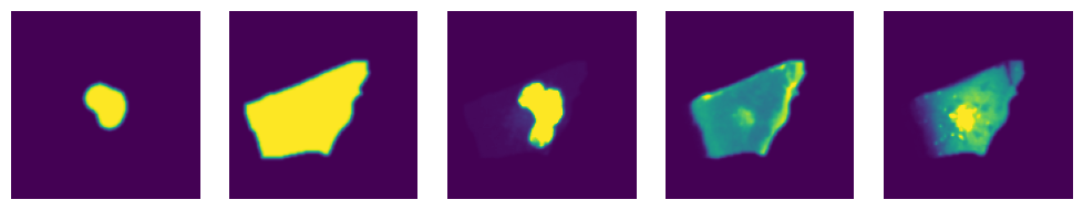
So if we want to look at the nth cell in the dataset we can first check which cellid was assigned to this cell by looking at the nth entry in the single_cell_index dataset and then get the extracted single-cell images from the single_cell_data dataset.
The extracted single-cell images represent the following information in this order:
nucleus mask 2. cytosol mask 3. nucleus channel 4. cytosol channel 5. other channels
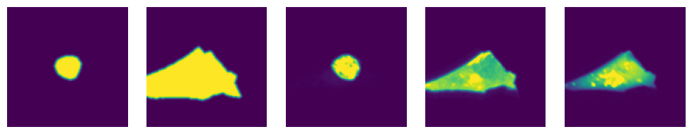
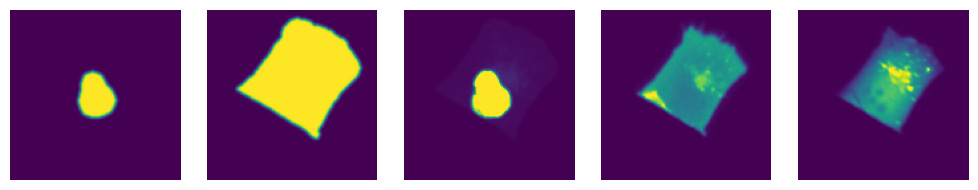
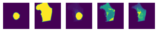
Here we will demonstrate with the 10th cell in the dataset.
[13]:
with h5py.File(f"{project_location}/extraction/data/single_cells.h5") as hf:
    index = hf.get("single_cell_index")
    images = hf.get("single_cell_data")

    print("cell id: ", index[10])

    image = images[10]

    fig, axs = plt.subplots(1, 5)

    for i, _img in enumerate(image):
        axs[i].imshow(_img)
        axs[i].axis("off")
cell id: [10 43]
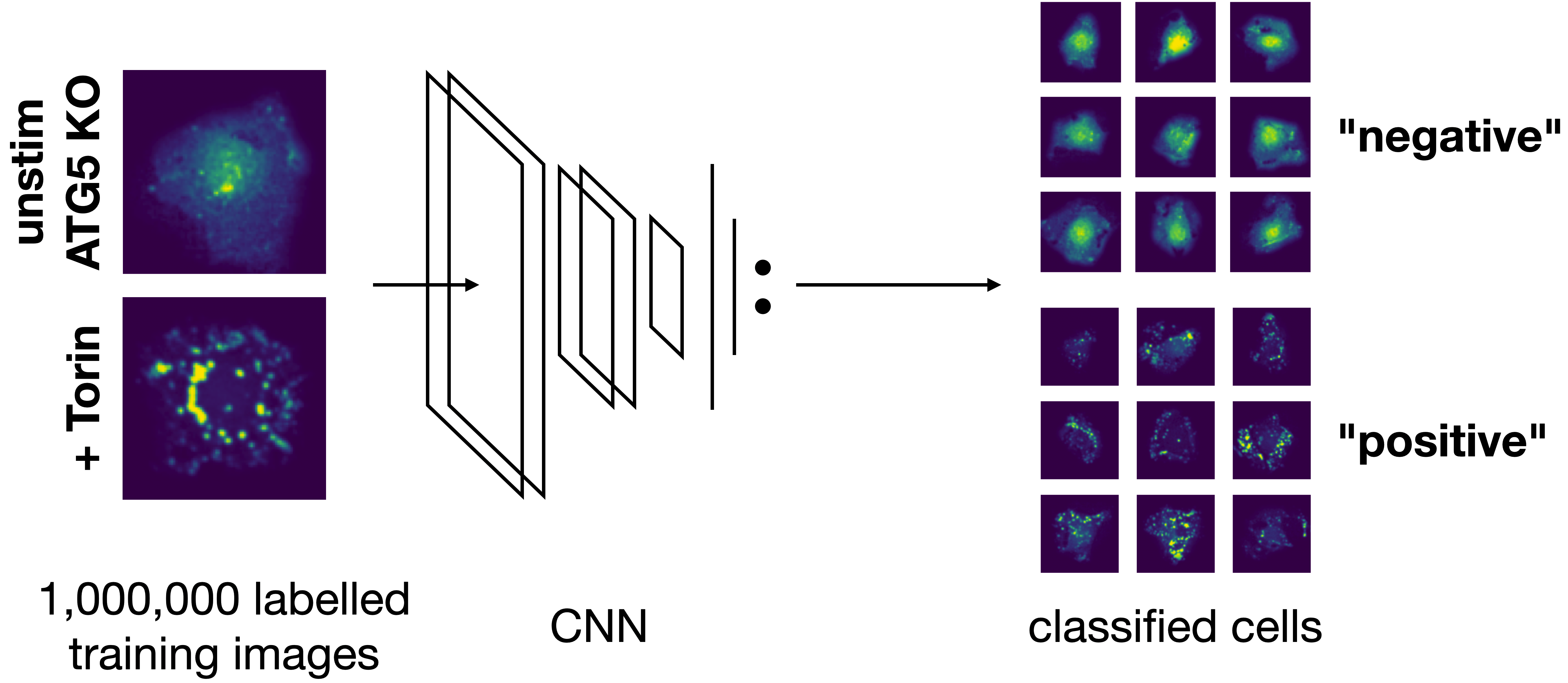
Classification of extracted single-cells
Next we can apply a pretained model to classify our cells within the scPortrait project.
Within the config.yml we specify which model should be used for inference and we can give it a name.
MLClusterClassifier:
    channel_classification: 4
    threads: 24 #
    batch_size: 900
    dataloader_worker: 0 #needs to be 0 if using cpu
    standard_scale: False
    exp_transform: False
    log_transform: False
    network: "autophagy_classifier2.1"
    classifier_architecture: "VGG2_old"
    screen_label: "Autophagy_15h_classifier2.1"
    epoch: "max"
    encoders: ["forward"]
    inference_device: "cpu"
Here e.g. we are using a pretrained model included within the scPortrait library autophagy_classifier2.1 and are naming the results from this model Autophagy_15h_classifier2.1.
Model overview:
The inference results will be written to a new folder generated under classification with this name.
If we want to use a model we trained ourselves that is not yet included within the scPortrait library we can simply replace the network name in the config with the path to the checkpoint file generated by pytorch.
[14]:
project.classify()
Using extraction directory: /Users/sophia/Documents/GitHub/scPortrait/example_data/example_1/project/extraction/data/single_cells.h5
[11/09/2024 17:11:14] Initialized temporary directory at /Users/sophia/Documents/GitHub/scPortrait/docs_source/pages/notebooks/MLClusterClassifier_s_af1va4 for MLClusterClassifier
[11/09/2024 17:11:14] Started MLClusterClassifier classification.
[11/09/2024 17:11:14] Created new directory for classification results: /Users/sophia/Documents/GitHub/scPortrait/example_data/example_1/project/classification/complete_Autophagy_15h_classifier2_1
[11/09/2024 17:11:14] CPU specified in config file but MPS available on system. Consider changing the device for the next run.
[11/09/2024 17:11:14] Model class defined as <class 'scportrait.tools.ml.plmodels.MultilabelSupervisedModel'>
Lightning automatically upgraded your loaded checkpoint from v1.5.5 to v2.4.0. To apply the upgrade to your files permanently, run `python -m pytorch_lightning.utilities.upgrade_checkpoint ../../../src/scportrait/pretrained_models/autophagy/autophagy2.1/VGG2_autophagy_classifier2.1.cpkt`
[11/09/2024 17:11:14] Model assigned to classification function.
[11/09/2024 17:11:14] Reading data from path: /Users/sophia/Documents/GitHub/scPortrait/example_data/example_1/project/extraction/data/single_cells.h5
[11/09/2024 17:11:14] Expected image size is set to [128, 128]. Resizing images to this size.
[11/09/2024 17:11:14] Dataloader generated with a batchsize of 900 and 10 workers. Dataloader contains 1 entries.
[11/09/2024 17:11:14] Starting inference for model encoder forward
[11/09/2024 17:11:14] Started processing of 1 batches.
[11/09/2024 17:11:17] finished processing.
[11/09/2024 17:11:17] Results saved to file: /Users/sophia/Documents/GitHub/scPortrait/example_data/example_1/project/classification/complete_Autophagy_15h_classifier2_1/inference_forward.csv
[11/09/2024 17:11:17] Table MLClusterClassifier_Autophagy_15h_classifier2_1_forward_nucleus written to sdata object.
[11/09/2024 17:11:17] Table MLClusterClassifier_Autophagy_15h_classifier2_1_forward_cytosol written to sdata object.
[11/09/2024 17:11:17] Results saved to file: /Users/sophia/Documents/GitHub/scPortrait/example_data/example_1/project/classification/complete_Autophagy_15h_classifier2_1/inference_forward.csv
[11/09/2024 17:11:17] GPU memory before performing cleanup: None
[11/09/2024 17:11:17] GPU memory after performing cleanup: None
[11/09/2024 17:11:17] Cleaned up temporary directory at <TemporaryDirectory '/Users/sophia/Documents/GitHub/scPortrait/docs_source/pages/notebooks/MLClusterClassifier_s_af1va4'>
looking at the generated results
The results are written to a csv file which we can load with pandas.
scPortrait writes the softmax results directly to csv as ln() for better precision. To transform these numbers back to the range between 0 and 1 we first need to apply the np.exp function.
[15]:
results = pd.read_csv(f"{project_location}/classification/complete_Autophagy_15h_classifier2_1/inference_forward.csv", index_col = None)
results.result_0 = np.exp(results.result_0)
results.result_1 = np.exp(results.result_1)

results
[15]:
| result_0 | result_1 | label | cell_id | |
|---|---|---|---|---|
| 0 | 0.017384 | 0.982615 | 0 | 12 |
| 1 | 0.000517 | 0.999483 | 0 | 13 |
| 2 | 0.806387 | 0.193613 | 0 | 15 |
| 3 | 0.146037 | 0.853963 | 0 | 18 |
| 4 | 0.896932 | 0.103068 | 0 | 33 |
| ... | ... | ... | ... | ... |
| 309 | 0.023494 | 0.976506 | 0 | 491 |
| 310 | 0.000234 | 0.999766 | 0 | 493 |
| 311 | 0.000014 | 0.999986 | 0 | 494 |
| 312 | 0.988722 | 0.011278 | 0 | 495 |
| 313 | 0.679858 | 0.320142 | 0 | 496 |
314 rows × 4 columns
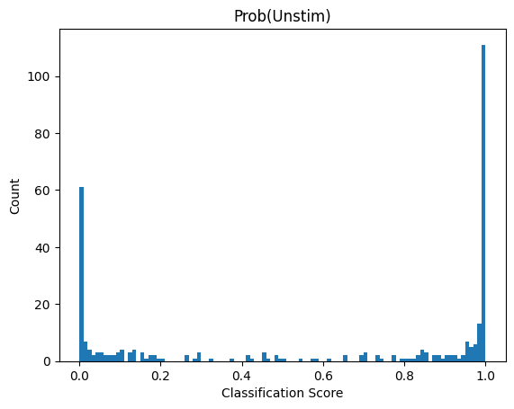
Depending on the model we used what result_0 and result_1 represent will vary. Here we used a binary classification model were class 1 was cells deficient in autophagy. So result_1 indicates the probability score that a cell has the label “autophagy off”. results_0 is simply 1 - result_1
If we look at the distribution in our dataset we can see that almost all cells are classified as “autophagy defective”. Since the input images were from unstimulated wt cells this matches to our expectation.
[16]:
plt.hist(results.result_1, bins = 100);
plt.title("Prob(Unstim)");
plt.xlabel("Classification Score");
plt.ylabel("Count");
Exporting Cutting contours for excision on the LMD7
scPortrait directly interfaces with our other open-source python library py-lmd to easily select and export cells for excision on a Leica LMD microscope.
Of note: this will require that the cells have been plates on a LMD compatible surface (like a PPS slide). scPortrait can of course also simply be used for data analysis procedures, then ignore this last step.
First we will select the cells we wish to excise based on their classification score. Here we have chosen a threadhold >= 0.99999 for bin1 and a threshold <= 0.9 for bin2.
[17]:
cell_ids_bin1 = results[results.result_1 >= 0.99999].cell_id.tolist()
cell_ids_bin2 = results[results.result_1 <= 0.9].cell_id.tolist()

print("number of cells to excise:",len(cell_ids_bin1) + len(cell_ids_bin2))
number of cells to excise: 177
The cells can then be allocated into different wells.
[18]:
cells_to_select = [{"name": "bin1", "classes": list(cell_ids_bin1), "well":"A1"},
                   {"name": "bin2", "classes": list(cell_ids_bin2), "well":"B1"},
                   ]
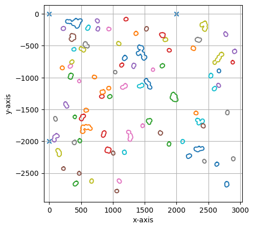
In addition to defining which cells we want to excise, we also need to pass the location of the calibration crosses so that we can transfer the image coordinate system into a cutting coordinate system. You can read up on this here.
To obtain the coordinates of your reference points simply open your stitched image in e.g. FIJI and navigate to the location of your reference points. Then write out the coordinates for each point.
[19]:
marker_0 = (0, 0)
marker_1 = (2000, 0)
marker_2 = (0, 2000)

calibration_marker = np.array([marker_0, marker_1, marker_2])
As with the previous methods, additional parameters can be passed to the selection function via the config.yml file which adapts the behaviour of how cutting shapes are generated. You can read up more on this here.
LMDSelection:
    processes: 20

    # defines the channel used for generating cutting masks
    # segmentation.hdf5 => labels => segmentation_channel
    # When using WGA segmentation:
    #    0 corresponds to nuclear masks
    #    1 corresponds to cytosolic masks.
    segmentation_channel: 0

    # dilation of the cutting mask in pixel
    shape_dilation: 16

    # number of datapoints which are averaged for smoothing
    # the number of datapoints over an distance of n pixel is 2*n
    smoothing_filter_size: 25

    # fold reduction of datapoints for compression
    poly_compression_factor: 30

    # can be "none", "greedy", or "hilbert"
    path_optimization: "hilbert"

    # number of nearest neighbours for optimized greedy search
    greedy_k: 15

    # hilbert curve order
    hilbert_p: 7
[20]:
project.select(cells_to_select, calibration_marker, segmentation_name = "seg_all_nucleus")
[11/09/2024 17:11:17] Initialized temporary directory at /var/folders/35/p4c58_4n3bb0bxnzgns1t7kh0000gn/T/./LMDSelection_5t71awp6 for LMDSelection
[11/09/2024 17:11:17] Selection process started.
No configuration for shape_erosion found, parameter will be set to 0
No configuration for binary_smoothing found, parameter will be set to 3
No configuration for convolution_smoothing found, parameter will be set to 15
No configuration for xml_decimal_transform found, parameter will be set to 100
No configuration for distance_heuristic found, parameter will be set to 300
No configuration for processes found, parameter will be set to 10
No configuration for join_intersecting found, parameter will be set to True
sanity check for cell set 0
cell set 0 passed sanity check
sanity check for cell set 1
cell set 1 passed sanity check
Calculating coordinate locations of all cells.
Processing cell sets in parallel
                  collecting cell sets:   0%|          | 0/2 [00:00<?, ?it/s]Convert label format into coordinate format
Convert label format into coordinate format
Conversion finished, performing sanity check.
Check passed
Check passed
Check passed
Merging intersecting shapes
Conversion finished, performing sanity check.
Check passed
Check passed
Check passed
Merging intersecting shapes
100%|██████████| 14/14 [00:02<00:00,  6.82it/s]
  1%|          | 2/163 [00:01<02:02,  1.31it/s]
Create shapes for merged cells
100%|██████████| 163/163 [00:02<00:00, 62.30it/s] it/s]
Create shapes for merged cells
creating shapes: 100%|██████████| 13/13 [00:02<00:00, 5.46it/s]
Calculating polygons
creating shapes: 100%|██████████| 72/72 [00:03<00:00, 21.88it/s]
Calculating polygons
calculating polygons: 100%|██████████| 13/13 [00:03<00:00, 3.80it/s]
Polygon calculation finished
Current path length: 19,006.29 units
Path optimizer defined in config: hilbert
Optimized path length: 19,006.29 units
Optimization factor: 1.0x
Figure(1000x1000)
                  collecting cell sets:  50%|█████     | 1/2 [00:10<00:10, 10.84s/it]
calculating polygons: 100%|██████████| 72/72 [00:02<00:00, 25.78it/s]
Polygon calculation finished
Current path length: 94,132.65 units
Path optimizer defined in config: hilbert
Optimized path length: 94,132.65 units
Optimization factor: 1.0x
Figure(1000x1000)
                  collecting cell sets: 100%|██████████| 2/2 [00:12<00:00,  6.11s/it]
===== Collection Stats =====
Number of shapes: 85
Number of vertices: 1,983
============================
Mean vertices: 23
Min vertices: 15
5% percentile vertices: 15
Median vertices: 19
95% percentile vertices: 44
Max vertices: 71
[0 0]
[      0 -200000]
[200000      0]
[11/09/2024 17:11:30] Saved output at /Users/sophia/Documents/GitHub/scPortrait/example_data/example_1/project/selection/bin1_bin2.xml
[11/09/2024 17:11:31] Cleaned up temporary directory at <TemporaryDirectory '/var/folders/35/p4c58_4n3bb0bxnzgns1t7kh0000gn/T/./LMDSelection_5t71awp6'>